
2.1. Method Overview and Basic Concepts
The concept of a fitness landscape is extensively utilized in fields such as biology, genetics, and optimization theory. It primarily describes the relationship between the solution space of an optimization problem and its corresponding fitness (or objective function) values. This concept draws inspiration from the undulating terrains found in nature to visually represent the quality of solutions, where each point signifies a potential solution, and the elevation of the point indicates the fitness value of that solution. Fitness Landscapes are particularly significant in genetic algorithms, evolutionary computation, and other heuristic search methods, as they offer an intuitive understanding of the characteristics inherent in a problem’s search space. By analyzing the Fitness Landscape, researchers and engineers can more effectively design and refine their optimization strategies to address complex optimization challenges.
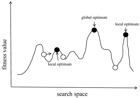
The concept of the fitness landscape is also applicable to the analysis of part surface morphology. Fitness landscape analysis has become an effective method for exploring the parameter information of part surface morphology. In the context of part surface morphology, each point on the local surface is treated as a potential solution. Consequently, the part surface morphology can be viewed as a surface with complex fitness values. By systematically searching this fitness landscape, the main features of the part surface morphology can be extracted. The main features of a fitness landscape include:
Height/Depth: In a fitness landscape, the height or depth of a point represents the fitness value of the corresponding solution. In minimization problems, valleys indicate optimal solutions, whereas in maximization problems, peaks signify optimal solutions.
Local Extremes: Local peaks or valleys on the fitness landscape correspond to local optimal solutions. These points can cause the search process to become easily trapped, hindering the discovery of the global optimum.
Global Extremes: The highest or lowest points on the fitness landscape represent the global optimal solutions.
Ruggedness: The ruggedness or irregularity of the fitness landscape reflects the complexity of the optimization problem. A highly rugged fitness landscape typically contains numerous local extremes, increasing the difficulty of locating the global optimal solution.
2.2. Mathematical Modeling of the Fitness Landscapes
In the context of optimization problems, the fitness landscape offers a visual framework for understanding the complexity of the search space, while heuristic algorithms serve as methods for identifying the optimal solution within this landscape. The definition of the fitness landscape is as follows.
A fitness landscape can be formally defined as a triplet , where denotes the solution space of the problem, encompassing all possible solutions. Depending on the specific problem, this space may be either continuous or discrete. The objective function is a mapping defined on the search space , assigning a metric value to each solution to evaluate its quality. The distance metric measures the distance between any two solutions and within the search space, serving as a function to quantify the distance or similarity between two points. This formalization provides a comprehensive framework for analyzing and navigating the complex morphology of the solution space, facilitating the design and application of effective heuristic algorithms for optimization.
Fitness landscape analysis offers an intuitive approach for optimizing low-dimensional functions. However, for optimization problems involving multi-dimensional variables, the complexity of the fitness landscape becomes challenging to represent through straightforward visualization. In such cases, Fitness-Distance Correlation (FDC) emerges as a crucial tool for quantifying and comprehending the ruggedness of the fitness landscape. FDC provides a systematic method for evaluating the relationship between the fitness of a solution and its distance to other solutions, thereby enhancing our understanding of the landscape’s structure and aiding in the development of more effective optimization strategies.
Fitness-Distance Correlation (FDC) is the correlation coefficient between the fitness of a solution and its distance within the solution space. It quantifies the ruggedness of the fitness landscape by calculating the statistical correlation between fitness and distance. In relatively smooth and continuous fitness landscapes, the fitness of a solution and its distance to the optimal point typically exhibit a strong correlation. In such cases, the FDC value tends to be large, usually close to 1 or −1. This indicates that points near the optimal solution generally possess higher fitness, while those farther from the optimal solution tend to have lower fitness. Conversely, in rugged and highly fluctuating fitness landscapes, the correlation between a solution’s fitness and its distance to the optimal point is weaker. In these scenarios, the FDC value is smaller, often approaching 0. This suggests that even solutions in close proximity to the optimal point may not exhibit ideal fitness levels, reflecting the presence of numerous local optima.
In practical scenarios involving complex part surface morphology models, determining the global optimum is often challenging and sometimes even infeasible. This difficulty arises because the exact location of the global optimum may be unknown or difficult to ascertain accurately due to the model’s complexity and computational limitations. In such cases, the traditional Fitness-Distance Correlation (FDC) metric, which relies on knowledge of the global optimum, may no longer be applicable. To address this limitation, an improved definition of FDC has been proposed, which utilizes optimal solutions sampled from a dataset constructed from a precise part surface morphology model, thereby replacing the reliance on the traditional global optimum.
where represents the corresponding value of point ; the average value of all sample points is represented as , that is, ; the Euclidean distance from to the optimal point is represented as , that is, ; and represents the average value of , that is, .
However, there are several limitations associated with using the FDC metric for evaluation. As discussed in the literature, the calculation of FDC relies on a limited sample set, which is often significantly smaller than the overall scale of the search space, potentially leading to biased results. Furthermore, according to Formula (1), the computation of FDC assumes that the position of the global optimum is known, thereby restricting its utility as a predictive tool and rendering it more suitable for post hoc verification. To address these limitations, an improved FDC metric approach is adopted in this study, which divides the search space into subintervals and analyzes the FDC values within each subinterval. Through extensive experiments, it is generally recommended that the FDC value be set between 0.4 and 0.7. Additionally, for black-box function optimization problems of part surface morphology, where gradient information of the unknown function is unavailable, determining the global optimum in advance is challenging. Therefore, this method samples surface information within each subinterval and designates the point with the highest fitness value among all sampled points as the local optimum for that region. This approach not only overcomes the limitations of the traditional FDC metric but also effectively elucidates the ruggedness of the surface.
Source link
Jinshan Sun www.mdpi.com