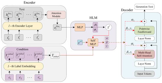
A Hierarchical Latent Modulation Approach for Controlled Text Generation

3.1. Hierarchical Latent Modulation Module

To further exploit latent variables and conditional information, we propose a network architecture based on conditional modulation, the Hierarchical Latent Modulation Module (HLMM), which provides the text generation task with more precise modulation of the feature distribution and modular output in the process of generating conditional information through a conditional modulation mechanism, providing higher control and flexibility for the text generation task. According to previous studies, latent variables can not only effectively capture the semantic information of the input text but also serve as additional conditions in the generation process, which are used to guide the diversity and consistency of the generation results. In addition, Memory Dropout further enhances the utilization of latent variables in the model [26].

As shown in Figure 1, the HLMM framework is based on the application of hierarchical latent spaces. It regulates the generated text by integrating latent variables and conditional information. The core idea is to utilize hierarchical latent variables to capture multi-level abstract features of the text and dynamically control the generation process by incorporating conditional information such as topics, sentiment, and semantic labels. The specific implementation is as follows: The original text and conditional information are encoded into continuous vector representations via an encoder. The conditional information (such as topics and sentiment labels) is transformed into low-dimensional dense vectors

Y_{e m b e d} \in R^{p}

via an embedding layer. The encoder further generates a distribution of multi-level latent variables

{z_{l}}_{l = 1}^{L}

. At each level of the latent space, the current latent variable

z_{l}

interacts with the previous layer’s latent variable

z^{< l}

through low-rank matrix factorization (LMF), where LMF maps the high-dimensional tensor to a low-dimensional representation

h^{l}

. This representation is then combined with the conditional information

Y_{e m b e d}

. To enhance the model’s use of latent variables, a random dropout of part of the conditional information is applied to encourage the model to rely more on the latent variables and avoid overfitting. Finally, modulation parameters are generated through the modulation network (HLM). The main formula is as follows:

$[α, γ, β] = Self MLP (Concat (LMF (z_{l}, z^{(< l)}), Y_{embed}))$

(10)

Among them,

α

and

γ

, and

β

are used as modulation parameters for scaling and offsetting the hidden state, respectively;

z_{l}

is the distribution feature of the latent variable in the l layer;

z^{< l}

denotes the latent variable in the previous layer; and

Y_{e m b e d}

is the embedded representation of the conditional information. The generated modulation parameters

γ

and

β

are embedded into the multi-head self-attention and feed-forward network modules of the decoder to modulate the hidden state distribution layer by layer, which is implemented as follows:

${\hat{h}}^{(l)} = γ^{(l)} ⊙ Norm (h^{(l)}) + β^{(l)}$

(11)

where ${\hat{h}}^{(l)}$ is the hidden state after modulation, the latent variable $z_{l}$ and the conditional information $Y_{e m b e d}$ are mapped to generate the modulation parameters, $Norm (\cdot)$ denotes the standard normalization operation, and ⊙ performs the element-by-element multiplication operation.

Through the proposed conditional modulation mechanism, the generative encoder is able to dynamically adjust the integration of conditional information during the generation process. This effectively alleviates the issue of the under-utilization of conditional information in traditional concatenation-based methods while also preventing mode collapse in generative models.

3.3. HLM-Based Method for Generating Conditional Modulation Parameters

The modulation parameters are crucial to subsequent generation. By generating conditional modulation parameters based on Hierarchical Latent Modulation (HLM), conditional information is explicitly embedded into the decoder in a fine-grained manner, thus realizing the deep control of the generation process. The specific implementation is as follows (Figure 2):

Conditional information is generated through the embedding layer to generate continuous feature representations

Y_{embed} \in R^{d}

, which are fused with the encoder output of the latent variable distribution

z_{l} \in R^{p}

, as well as with the parameters of the latent variable learning before

z_{l}

, where in order to better obtain the feature information of the latent variables, low-rank tensor product fusion is employed [26] as

LMF (z_{l}, z^{(< l)})

, with the following formula:

$h^{(l)} = LMF (z_{l}, z^{(< l)}) = (\sum_{j = 1}^{r} W_{v}^{(l, j)} z_{l}) \circ (\sum_{j = 1}^{r} W_{z}^{(l, j)} z^{(< l)})$

(24)

where $z_{l} \in R^{p}$ is the current latent variable distribution, $z_{l} \in R^{p}$ is the current latent variable distribution, $z^{< l} \in R^{p}$ is the characterization of the latent variables in the previous layer, $W_{v}^{(l, j)} \in R^{d \times p}$ corresponds to the $j - t h$ projection matrix of $z_{l}$ , $W_{z}^{(l, j)} \in R^{d \times p}$ corresponds to the $j - t h$ projection matrix of $z_{l}$ , and ∘ denotes the element-by-element product.

The tensor outer product explicitly expresses the high-order interactions between latent variable features. Given multiple latent variable feature vectors

{z_{l}}_{l = 1}^{L}

, the high-order tensor

Z = ⨂_{l = 1}^{L} z_{l}

is generated through the outer product, capturing the combined information from the multi-layer latent variables. This high-order tensor is then mapped to a lower-dimensional output space h through a linear transformation

h = W \cdot Z + b

for subsequent tasks. However, the dimension of the high-order tensor is usually large, and directly storing these tensors leads to a significant increase in computational cost. Therefore, low-rank approximation is used, as shown by the formula

$W \approx \sum_{i = 1}^{r} ⨂_{l = 1}^{L} w_{l}^{(i)}$

(25)

where r is the rank, much smaller than the original dimension. The low-rank approximation significantly reduces the number of parameters, from $O (\prod_{l = 1}^{L} d_{l})$ to $O (r \sum_{l = 1}^{L} d_{l})$ . Furthermore, through parallel decomposition, both the input tensor Z and the weight tensor W can be decomposed into specific low-rank factors, i.e., $Z = ⨂_{l = 1}^{L} z_{l}$ and $W \approx \sum_{i = 1}^{r} ⨂_{l = 1}^{L} w_{l}^{(i)}$ . The output h can then be computed directly as

$h = \sum_{i = 1}^{r} (⨀_{l = 1}^{L} w_{l}^{(i)} \cdot z_{l})$

(26)

where ⨀ represents element-wise multiplication. This reduces the computational complexity from $O (d_{h} \prod_{l = 1}^{L} d_{l})$ to $O (d_{h} \times r \times \prod_{l = 1}^{L} d_{l})$ , avoiding the explicit generation and storage of high-dimensional tensors Z and W, thus improving computational efficiency.

Low-rank fusion (LMF) makes full use of the latent variables $z_{l}$ and the feature information from the previous layers $z^{< l}$ . By designing learnable parameter matrices $W_{v} \in R^{d \times d}$ and $W_{z} \in R^{p \times d}$ , it enables information transmission and sharing between different layers, ensuring that these parameters are shared across all positions $(i)$ , but not across layers $(l)$ . This design ensures that the latent variable information at each layer can be transformed through a unified projection. This approach effectively builds deep dependencies between layers and helps latent variable interactions across different layers through shared parameters. Not only does this enhance the flow of information across layers, but it also improves the model’s memory capacity for historical features and reduces the risk of overfitting.

The information in

h^{l}

after low-rank fusion is dense, allowing for the better utilization of conditional information. Furthermore, through element-wise multiplication, gradient calculations depend only on the corresponding dimensions of the latent variables, reducing the risk of gradient vanishing or explosion. Specifically, the gradient is

$\frac{\partial z_{l}}{\partial h} = \sum_{j = 1}^{r} W_{v}^{(l, j)} \circ (\sum_{j = 1}^{r} W_{z}^{(l, j)} z^{(< l)})$

(27)

Compared with fully connected layers, this gradient computation is more stable and has the structure shown below (Figure 3).

The fusion latent variable $h^{l}$ and the condition information $Y_{e m b e d}$ are spliced to form the HLM input feature $Concat (h^{l}, Y_{embed})$ to obtain the semantic features and condition information, and the spliced input feature x is convolved in one dimension to extract the local continuous features to capture the context information in the time dimension; at the same time, the dependency relationship between the features is enhanced to make the semantic expression more recognizable. In addition, to prevent the model from overly relying on conditional information during the training process, a dropout mechanism is introduced to discard specific conditional information. Specifically, some of the conditional information $Y_{e m b e d}$ is randomly dropped, thereby forcing the model to rely more on the latent variables $h^{l}$ rather than solely depending on the conditional information for generation. This dropout mechanism helps promote the diversification of the latent variables’ expression during the generation process, preventing the model from relying exclusively on conditional information while neglecting the latent features.

We use the Multi-Layer Perceptual (MLP) Network to generate the parameters

α

(scaling factor),

γ

(scaling factor), and

β

(offset). The MLP is implemented with the following formula:

$MLP (x) = W_{2} \cdot ReLU (W_{1} \cdot x + b_{1}) + b_{2}$

(28)

where $x = Concat (h^{l}, Y_{embed})$ , $W_{1} \in R^{h \times (p + d)}$ , $W_{2} \in R^{2 d \times h}$ , and $b_{1}$ and $b_{2}$ are biases.

Next, through Hierarchical Latent Modulation (HLM), a fine-grained embedding strategy is used to tightly integrate the conditional information with the semantic features, and the modulation parameters are generated, enabling the explicit modulation of the distribution and expression of the features, thus enhancing the decoder’s in-depth control over the generation process.

3.4. HLM-Based Method for Generating Conditional Modulation Parameters

At each layer of the decoder, the generated modulation parameters

α

γ

, and

β

are normalized by introducing Hierarchical Latent Modulation (HLM) with the following equations:

${\hat{h}}^{(l)} = γ^{(l)} ⊙ Norm (h^{(l)}) + β^{(l)}$

(29)

where $h^{(l)}$ is the hidden state of decoder layer l and $Norm (\cdot)$ denotes layer normalization for the standardized hidden states, as follows:

$Norm (h^{(l)}) = \frac{h^{(l)} - μ}{σ}, μ = \frac{1}{d} \sum_{i = 1}^{d} h_{i}^{(l)}, σ = \sqrt{\frac{1}{d} \sum_{i = 1}^{d} {(h_{i}^{(l)} - μ)}^{2}}$

(30)

where $μ$ and $σ$ are the mean and variance, respectively; $γ^{(l)}$ and $β^{(l)}$ are a scaling factor and an offset parameter, respectively, jointly generated from conditional information and latent variables; and ⊙ denotes element-by-element multiplication.

HLM generates conditional modulation parameters to adjust the feature distribution of the hidden states, allowing conditional information to effectively participate in the generation process. The primary role of the normalization operation is to standardize each feature of the hidden states, ensuring that the mean is 0 and the variance is 1. This guarantees consistency across the layers of the input hidden states, preventing issues such as vanishing or exploding gradients. By doing so, the model avoids learning difficulties that arise from inconsistent feature scales during training. The modulation parameters $γ^{(l)}$ and $β^{(l)}$ at each layer adjust the feature distribution of the hidden states, precisely controlling the scaling and shifting of the hidden states. Specifically, $γ^{(l)}$ controls the scale of each feature, determining the magnitude of the feature values, while $β^{(l)}$ controls the shift of each feature, ensuring that the features can adapt to changes in both the conditional information and the latent variables during the generation process.

The conditional modulation parameters are generated by HLMM to adjust the feature distribution of the hidden state so that the conditional information can effectively participate in the generation process, which acts with the cross-attention (MSA) module and the feed-forward network (FFN) module, respectively, for scaling and biasing, as follows:

${\hat{h}}_{attn} = a_{msa}^{(l)} \cdot A_{Attn}^{modulated} + h^{(l)}$

(31)

where $a_{msa}^{(l)}$ is the generated scaling factor for adjusting the amplitude of the output of the cross-attention module, $A_{attn}^{modulated} = γ_{msa}^{(l)} ⊙ Norm (A_{attn}) + β_{msa}^{(l)}$ is the output of the cross-attention distribution, and $h^{(l)}$ is the input hidden state of the module.

${\hat{h}}_{FFN} = a_{mlp}^{(l)} \cdot A_{FNN}^{modulated} + {\hat{h}}_{attn}$

(32)

where $a_{mlp}^{(l)}$ is the generated scaling factor for adjusting the amplitude of the output of the feed-forward network module, $A_{FFN}^{modulated} = γ_{mlp}^{(l)} ⊙ Norm (h_{FFN}) + β_{mlp}^{(l)}$ is the output of the cross-attention distribution, and ${\hat{h}}_{attn}$ is the output of the cross-attention module.

The embedding of modulation parameters enables the model to fully utilize conditional information and latent variable features during the generation process, adjusting the feature distribution in a detailed and precise manner.

Source link

Jincheng Zou www.mdpi.com

Greenberg News

A Hierarchical Latent Modulation Approach for Controlled Text Generation

3.1. Hierarchical Latent Modulation Module

3.3. HLM-Based Method for Generating Conditional Modulation Parameters

3.4. HLM-Based Method for Generating Conditional Modulation Parameters

Greenberg

3.1. Hierarchical Latent Modulation Module

3.3. HLM-Based Method for Generating Conditional Modulation Parameters

3.4. HLM-Based Method for Generating Conditional Modulation Parameters

Related Posts

Effect of Ti and TiNb Microalloying on Microstructures and Mechanical Properties of 2200 MPa Low-Alloy Ultra-High-Strength Steels

Environmental Factor – July 2020: Reductions in animal testing celebrated at national meeting

How Ancient Practices Can Solve Modern Sustainability Problems

Greenberg