A Lightweight Framework for Rapid Response to Short-Term Forecasting of Wind Farms Using Dual Scale Modeling and Normalized Feature Learning

1. Introduction

Against the backdrop of increasing energy demand today, the widespread use of traditional energy is further exacerbating the energy crisis and promoting the deterioration of the greenhouse effect [1]. Therefore, people are turning their attention to renewable energy, especially wind energy. According to the 2022 Global Wind Energy Report released by the Global Wind Energy Council (GWEC), the global wind energy installed capacity is expected to increase by 680 million kilowatts from 2023 to 2027 [2]. This indicates that wind energy, as an environmentally friendly and widely distributed renewable energy source, is being actively promoted. However, the inherent randomness and instability of wind resources result in a high degree of uncertainty and unpredictability in wind power generation, posing significant challenges to the stable operation of the power grid and electricity dispatching [3]. Accurate short-term forecasting can help grid operators efficiently manage the power resources of wind farms, improving wind energy utilization and reducing operational costs. Moreover, the current real-time forecasting of wind farms places high demands on model forecasting efficiency; therefore, accurate and efficient wind power forecasting is crucial to meet these challenges.

Current models applied in the field of wind power forecasting mainly include physical models, statistical models, machine learning models, and deep learning models. Physical models use hydrodynamics and thermodynamics to simulate the interaction between wind and the atmosphere; by incorporating factors such as terrain and landforms and solving physical equations, they predict wind speed and direction at specific locations and heights. The output power of the wind farm is then calculated based on the power curve of the wind turbines [4]. However, physical models typically require large computational resources and real-time data, making them unsuitable for short-term forecasting [5]. On the other hand, statistical models such as Autoregressive (AR) [6], Autoregressive Moving Average (ARMA) [7], and Autoregressive Integrated Moving Average (ARIMA) [8] predict by establishing mathematical relationships between historical meteorological data and wind power. Wang et al. proposed a forecast error compensation method based on the ARIMA model to improve forecasting accuracy [9]. However, statistical models may be limited in handling complex non-stationary wind power sequences due to assumptions they are based on, such as linear distribution, which can lead to underfitting and lower forecasting accuracy [10].

In recent years, many classic machine learning techniques have been applied to short-term wind power forecasting, including Support Vector Machine (SVM) [11,12], Random Forests (RF) [13], Extreme Gradient Boosting (XGBoost) [14], and Extreme Learning Machine (ELM) [15]. Compared to statistical methods, machine learning models are able to effectively model the nonlinear relationships between wind power data at different time points [16]. In addition, deep learning has become a popular technology in the field of wind power forecasting with its excellent data feature mining ability and complex network architecture [17]. Among them, the commonly used deep learning models include CNN [18], TCN [19], RNN [20], and its two variants, LSTM [21] and GRU [22], etc. Hybrid models usually have better forecasting performance than a single model due to the integration of the unique advantages of different models [23]. Zhao et al. [24] employed variational mode decomposition to reduce the volatility of the original wind speed series. The decomposed subsequences, combined with the original wind power series, are then fed into a CNN-GRU hybrid model for short-term wind power forecasting.

Moreover, in recent years, the model based on the attention mechanism has demonstrated its powerful performance in various time series forecasting tasks, including wind speed forecasting [25], solar irradiance forecasting [26], and traffic flow forecasting [27]. This mechanism typically focuses on key features that significantly impact the forecasting results to address time series forecasting problems [28]. The Transformer [29], with its encoder-decoder structure and self-attention mechanism, can capture complex time-dependency patterns and correlations among different sequential variables, thereby achieving better forecasting results. Building upon this, the model based on the attention mechanism has been gradually introduced into the field of wind power forecasting and has achieved notable success. For instance, Sun et al. [30] proposed a short-term wind power forecasting method using the Transformer that considers spatio-temporal correlations. Gong et al. [31] combined the strengths of TCN and Informer, significantly enhancing the accuracy of wind power forecasting. In addition, Xiang et al. [32] utilized the multi-head self-attention mechanism of Vision Transformer to fully exploit the complex nonlinear relationships among input data, thereby improving the accuracy of ultra-short-term wind power forecasting. Liu et al. [33] proposed an interpretable Transformer model integrating decoupled feature-temporal self-attention and variable-attention networks and enhanced wind power prediction accuracy through multi-task learning.

As mentioned earlier, Transformers and their variants have achieved high accuracy in wind power forecasting. However, due to the reduction of correlation between distant data points in the sequence, it is difficult for the Transformer to adequately understand the global information of the sequence [34]. Additionally, the time complexity of Transformers grows quadratically with the increase in time series length [35]. Based on these considerations, Zeng et al. [36] questioned the applicability of such models as Transformer in the field of time series forecasting and proposed a simple single-layer linear model, DLinear, which decomposes the data into a moving average component and a seasonal trend component and then applies a single linear layer to the two components, respectively. DLinear is experimentally demonstrated to be superior to the complex Transformer-based model in terms of prediction accuracy and computational efficiency. Meanwhile, Zhang et al. [37] proposed a lightweight multivariate forecasting architecture based on stacked multi-layer perceptrons (MLPs) called LightTS, further advancing research in lightweight forecasting. This model converts one-dimensional sequences into two-dimensional tensors through different sampling methods, allowing it to focus separately on analyzing short-term local variations and long-term global variations and then uses the MLP to learn the sequential features within these tensors, achieving improved forecasting accuracy while significantly reducing computational complexity. Summing up the previous analysis, from the perspective of forecasting accuracy and efficiency, lightweight models have a promising application prospect in time series modeling.

We have observed that training complex network models and tuning their parameters typically require significant computational resources and time, especially for Transformer-based models, which often have millions of parameters. This makes their application in resource-limited environments (such as edge computing nodes or remote wind farms) challenging [38]. In contrast, lightweight models are more practical due to their lower computational resource requirements. To ensure the load safety of wind turbines, the control system needs to adjust the pitch angle and rotational speed of the blades in response to changes in wind speed. However, due to delays in the control system, this can lead to excessive loads on the turbine. Moreover, wind speed measurement devices such as lidar are sensitive to weather conditions, making it difficult to provide reliable wind measurements. Therefore, deploying lightweight prediction models to provide short-term wind speed forecasts for each turbine is a technological solution that can help reduce the load on the turbines. Furthermore, lightweight models generally offer faster computation speeds. In applications that require forecasting wind power for a specific region [39], they can quickly process and predict the output of wind power clusters consisting of multiple wind farms across a large spatial area, which is crucial for grid scheduling of wind resources. Therefore, lightweight wind power forecasting models are of significant importance for real-time predictions in wind farms. By simplifying the structure and reducing the number of parameters, they maintain a good balance between performance and lightweight design, accelerate the wind farm’s response time and update frequency to fluctuations in wind power generation, and reduce operational costs. In the field of wind power forecasting, Lai et al. [40] developed a lightweight spatiotemporal wind power forecasting network, which synchronously learns spatiotemporal representations through the spatial layer and asynchronously learns temporal representations through the asynchronous spatial layer. They also used MLP to update wind power information along the temporal dimension, improving the efficiency of capturing wind power’s spatiotemporal relationships. Moreover, since online learning emphasizes a model’s ability to learn from new data in real-time and continuously update itself, online learning models often require simpler structures. Zhong et al. [41] introduced external time-related data and designed a lightweight parallel network to process these external data, mitigating information transmission degradation and enhancing online forecasting performance. In this paper, based on the great potential of simple linear models and the limitations of complex network models, we decide to introduce LightTS, a lightweight deep learning architecture that utilizes MLP in time and channel dimensions and thus achieves a lightweight model structure. However, LightTS does not adapt well to the characteristics of wind power data due to the inherent non-stationarity of wind power sequences [42]. Therefore, we have decided to make further improvements based on LightTS.

In fact, the wind power series are typical time series with nonlinear and dynamic characteristics, and the value of each time step is affected by the past moments. This dependency arises because wind speed at a given moment is affected by various physical factors and temporal dynamics, such as atmospheric inertia, turbulence, and changing weather patterns, which introduce correlations between consecutive wind speed measurements. Specifically, wind speed time series often exhibit significant autocorrelation, meaning there is a statistical relationship between the current and past wind speeds [43]. Since wind speed affects the power generation of wind turbines, it creates a time dependency between wind power values at different moments. Although shallow models possess excellent nonlinear representation capabilities for time series modeling, they usually model the relationship between the input measurements and future predicted values of wind power series based on static space [44]. This approach may overlook the dynamic relationships that change over time between samples, leading to the patterns observed by the model in the past becoming inapplicable for the future, thus impacting forecasting accuracy. Based on this situation, we were inspired by the idea of RevIN [45] and proposed a normalization feature learning block, which is used as a key component of the proposed model to process sequence features. This block mitigates the negative impact of dynamic characteristics on model forecasting by removing dynamic statistical properties from the sequence features through preprocessing. Then, it applies MLPs in the temporal and channel dimensions for feature learning.

Considering the computational complexity of the model and the impact of the non-stationary nature of wind power data, we explore the potential of simple and lightweight deep learning network structures in the field of short-term wind power forecasting. The main contributions of this paper are as follows:

(1) To reduce the impact of dynamic relationships in wind power series on the forecasting performance of the model, we have proposed a Normalized Feature Learning Block (NFLBlock). This block removes the time-varying dynamic characteristics from the sequence features, allowing for better utilization of the stacked MLP structure for information interaction in both temporal and channel dimensions.

(2) To address the issues of overfitting and high training time costs associated with complex forecasting models, which hinder quick and accurate responses for real-time wind power forecasting in wind farms, we have developed a lightweight normalized feature learning forecasting model, NFLM, to achieve short-term multivariate wind power forecasting. This model is based on a stacked multi-layer perceptron architecture and, through continuous and interval sampling, can fully exploit the local and global dependencies in wind power sequences across different time scales.

(3) We tested the NFLM model at two wind farms in Guangxi, China. The results show that NFLM outperforms existing complex wind power forecasting models based on Transformers and recurrent structures in terms of forecasting accuracy. Additionally, NFLM maintains low computational and parameter requirements across all forecasting horizons.

The rest of this paper is organized as follows: we briefly introduce the framework of NFLM and its key components in Section 2. Section 3 conducts relevant experiments and discusses the model’s forecasting effectiveness and forecasting efficiency. In Section 4, we summarize our work and outlook for the future.

2. Materials and Methods

2.1. Overview of NFLM

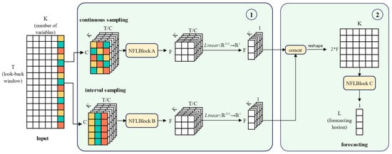
In the current field of wind power forecasting, many models employ complex neural network structures to capture the intricate temporal patterns of wind power series. However, such complex structure increases the computational complexity of the model and requires more computational resources and time. Additionally, due to the intermittency and volatility of wind resources, wind power series often contain dynamic features with time variability, leading to patterns in future data that differ from those historically observed. This discrepancy makes it challenging for models to adapt the information learned during the training phase to unknown test data, thereby affecting forecasting accuracy. To address these challenges, we constructed NFLM, a lightweight forecasting model for multivariate wind power forecasting, and proposed a Normalized Feature Learning Block (NFLBlock) inspired by the RevIN model for learning temporal features in the series. As shown in Figure 1, in the first part of the model, we perform continuous and interval sampling on the original series, generating two different time-scale input sequences that are processed independently. The dynamic statistical properties of these sequences are first removed in NFLBlock, and then the MLP stack structure is used to perform feature projection in both time and channel dimensions. After that, the statistical properties are restored back to these features to capture the local and global temporal dependencies in the series. In the second part of the model, we concatenate the features extracted from the first part, and the NFLBlock is used to learn correlations between different time series variables and make forecasting. The two sampling methods and normalization feature learning modules in NFLM will be detailed in the following sections.

2.2. Continuous Sampling and Interval Sampling

An important characteristic of time series is that down-sampling time series can still largely preserve the position information within the series. However, traditional sampling methods usually remove some units within the time step, leading to irreversible information loss. Based on this observation, we adopt continuous and interval sampling without removing any base units. The advantage of this sampling strategy is that it transforms the original series into two forms with different feature distributions, enabling the model to extract sequence features at different time scales so as to comprehensively capture the change patterns of wind power data. Specifically, continuous sampling can better reflect the local view of the wind power series, while interval sampling focuses more on the global view of the series. By employing both sampling strategies simultaneously, the model can deeply mine hidden features in wind power data from different perspectives.

In multivariate wind power forecasting, we assume that

K, T

and

L

correspond to the number of variables, the length of the input sequence, and the length of model forecasting, respectively. When the time step length is

t

, given input sequence

X_{t} = i = (1, 2, \dots K)

, our down-sampling method transforms the time series into

K

two-dimensional matrices with dimension

C \times T / C

, This means, for a chosen subsequence length

C

, continuous sampling will continuously select

C

tokens to form a subsequence each time. Thus, for each input sequence

X_{t} \in ℝ^{T}

of length

T

, it is down sampled into

T / C

non-overlapping subsequences to obtain the two-dimensional matrix

X_{t}^{c o n} \in R^{C \times T / C}

, where the

j – t h

column formed by continuously sampling the sequence of the

i – t h

feature variable is:

${X_{t}^{c o n}}_{• j} = x_{t - T + 1 + (j - 1) \cdot C}^{(i)}, x_{t - T + 2 + (j - 1) \cdot C}^{(i)}, \dots, x_{t - T + j \cdot C}^{(i)}$

(1)

In interval sampling, a fixed interval is used to select

C

tokens each time to form a subsequence. Similarly, the

j – t h

column of the two-dimensional matrix obtained by interval sampling of the

i – t h

feature variable sequence is represented as follows:

${X_{t}^{int}}_{• j} = x_{t - T + j}^{(i)}, x_{t - T + j + ⌊T / C⌋}^{(i)}, x_{t - T + j + 2 \cdot ⌊T / C⌋}^{(i)}, \dots, x_{t - T + j + (C – 1) \cdot ⌊T / C⌋}^{(i)}$

(2)

The strategies of continuous and interval sampling can help the model learn different temporal patterns. Specifically, continuous sampling divides the original sequence into several short-term subsequences, providing a local perspective for the model, thereby aiding in the capture of short-term temporal patterns. Interval sampling focuses on the global information, where the model learns trends over longer time spans on sparsely spaced slices. Notably, this down-sampling does not discard any data points from the original sequence but rearranges them into non-overlapping subsequences. In the following content, we will detail how to further explore effective time series features based on these sampled subsequences using the NFLBlock.

2.3. Reversible Instance Normalization

We consider the multivariate forecasting problem of predicting future wind power through multiple historical meteorological features and wind power. This section introduces reversible instance normalization, which can remove time-varying statistical properties from the wind power series features, enabling the temporal patterns learned during the training phase to be more applicable to test data, thereby improving the predictive capability of the model. Generally, RevIN operations can be applied to any chosen layer to perform instance normalization and perform the inverse normalization at a symmetrical position in another layer. For the input sequence

X_{t} \in ℝ^{T}

, we first calculate the mean

ℤ_{t} [x_{k t}^{(i)}]

and variance

V a r [x_{k t}^{(i)}]

of the input sequence using each sample

x_{k \cdot}^{(i)} \in ℝ^{T}

within it.

$\begin{array}{l} ℤ_{t} [x_{k t}^{(i)}] = \frac{1}{T} \sum_{j = 1}^{T} x_{k j}^{(i)} \\ V a r [x_{k t}^{(i)}] = \frac{1}{T} \sum_{j = 1}^{T} {(x_{k j}^{(i)} - ℤ_{t} [x_{k t}^{(i)}])}^{2} \end{array}$

(3)

These statistics are used for scaling and shifting, followed by normalizing the original data using these statistics:

${\hat{x}}_{k t}^{(i)} = γ_{k} (\frac{x_{k t}^{(i)} - ℤ_{t} [x_{k t}^{(i)}]}{\sqrt{V a r [x_{k t}^{(i)}] + ε}}) + β_{k}$

(4)

$γ, β \in ℝ^{K}$ is a learnable affine parameter vector. After normalization, the mean and variance of the sequence tend to be stable and consistent, thus mitigating the impact of dynamic factors. As a result, the normalization layer ensures that the model effectively identifies variation within the sequence when faced with inputs that have stable mean and variance.

Next, the transformed wind power series features

{\hat{x}}^{(i)}

is used as the input to the module for feature extraction on different dimensions. However, we notice that such input data differs in statistical properties from the original distribution. A module relying solely on normalized input data may not adequately capture the original features of the data. Therefore, the inverse normalization operation is performed at a symmetrical position to the normalization layer. The purpose of this operation is to reintroduce the statistical properties removed during input back into the output of the module so that the wind power value predicted by the model more closely matches the actual value of the original wind power series. We inverse normalize the output of the module based on Equation (4) using inverse arithmetic thinking:

${\hat{y}}_{k t} = \sqrt{V a r [x_{k t}] + ε} \cdot (\frac{{\tilde{y}}_{k t} - β_{k}}{γ_{k}}) + ℤ_{t} [x_{k t}]$

(5)

Herein, $\tilde{y}$ represents the wind power series obtained after feature projection by the module, and after reintroducing the original dynamic characteristics, now is the final output value of the module. Our focus is on the dynamic properties of the input data, including statistical properties such as mean $μ$ , variance $σ^{2}$ , and the learnable affine parameters $γ$ and $β$ . In the RevIN framework, normalization and inverse normalization layers are placed at symmetrical positions in the network, with the former used to remove statistical features and the latter to recover them. Through normalization, the original data is transformed into a zero-mean distribution, which reduces the distribution difference between different instances. To restore this removed information in the output, RevIN employs an inverse normalization process at the output layer, reintroducing the previously eliminated dynamic information. This enables each sample to regain its original distribution properties, beneficial for the final forecasting target computation, making the model’s forecasting more accurate.

2.4. Normalized Feature Learning Block

Figure 2 shows the structure of the Normalized Feature Learning Block (NFLBlock), which is a key component in the NFLM model for feature extraction and forecasting. Its main function is to realize information exchange of input features in the time dimension and channel dimension. The input of the NFLBlock is a two-dimensional matrix with a time dimension of

H

and a channel dimension of

W

. To alleviate the negative impact of dynamic characteristics in wind power series data on forecasting, we first perform an instance normalization operation on this matrix and then perform temporal projection and channel projection through the MLP stacked structure, producing a two-dimensional matrix of shape

F \times W

, where

F

represents the hyperparameter for the number of output feature dimensions. The output matrix can be regarded as the features obtained after the feature projection of the input matrix.

We denote the input matrix with

R = {(r_{i j})}_{H \times W}

, where the

i – t h

row is represented as

r_{i \cdot} = (r_{i 1}, r_{i 2}, \dots, r_{i W})

i = (1, 2, \dots, H)

and the

j – t h

column is represented as

r_{\cdot j} = (r_{1 j}, r_{2 j}, \dots, r_{H j})

j = (1, 2, \dots W)

. First, the instance normalization layer is applied to normalize the input two-dimensional matrix

R^{H \times W}

to obtain

R = {({r^{'}}_{i j})}_{H \times W}

, thereby removing the dynamic statistical characteristics in the series:

${({\hat{r}}_{i j})}_{H \times W} = R I N {(r_{i j})}_{H \times W}$

(6)

Then, an MLP of

ℝ^{H} \to ℝ^{F^{'}} (F^{'} < < F)

is used to implement feature projection from high dimension to low dimension on each column, which we refer to as temporal projection (Equation (7)). Subsequently, another MLP of

ℝ^{W} \to ℝ^{W}

is employed to perform channel projection on each row (Equation (8)):

${r^{t}}_{\cdot j} = M L P ({\hat{r}}_{\cdot j}), j = 1, 2, \dots, W$

(7)

${r^{c}}_{i \cdot} = M L P ({r^{t}}_{i \cdot}), i = 1, 2, \dots, F^{'}$

(8)

Temporal projection and channel projection are feature transformations performed, respectively, on the time and channel dimensions. In the next step, we will use an MLP of

ℝ^{F^{'}} \to ℝ^{F}

to perform output projection on each column, projecting feature dimension

F^{'}

F

${r^{o}}_{\cdot j} = M L P ({r^{c}}_{\cdot j}), j = 1, 2, \dots W$

(9)

For the NFLBlock, relying solely on normalized data

{(r_{i j}^{'})}_{H \times W}

is insufficient to fully capture the distribution characteristics of the original data. Therefore, we perform an inverse normalization operation at the symmetrical output position of this module, explicitly restoring the statistical properties removed from the input data back into the module output:

${\tilde{r}}_{i j} = I R I N {({r^{o}}_{i j})}_{F \times W}$

(10)

where ${\tilde{r}}_{i j}$ represents the final output of the NFLBlock. For its input dimensions $H$ and $W$ , in the first part of NFLM, $H$ and $W$ correspond to the length of the subsequence $C$ and the number of divided subsequences $T / C$ , respectively. In the second part, $H$ corresponds to $2 \times F$ , the sum of the output feature dimensions extracted in the first part, and $W$ represents the number of sequence variables $N$ .

In the NFLBlock architecture, RevIN aims to handle the dynamic statistical properties in the input matrix, so that the feature distribution of the training and test data is more stable. Firstly, the input sequence is normalized, and then the inverse normalization layer performs a reverse normalization operation on the module output to the same extent as the normalization layer, thereby restoring the statistical information from the original distribution back into the module output. NFLBlock repeatedly performs channel projection on each time step, and when processing longer time series, the computational complexity significantly increases. To reduce computational costs, NFLBlock adopts a bottleneck structure. It is called a “bottleneck” because a smaller intermediate length $F^{'}$ is introduced into the structure, which is much smaller than both $H$ and $F$ . That is, the length $H$ of the input sequence is first projected $F^{'}$ through a temporal projection layer. Then, channel projection is performed $F^{'}$ times to realize information exchange, and finally, the output projection layer projects the features of length $F^{'}$ back to the required output length $F$ . The bottleneck structure greatly reduces the amount of repetitive channel projection calculation.

Source link

Yan Chen www.mdpi.com

Greenberg News

A Lightweight Framework for Rapid Response to Short-Term Forecasting of Wind Farms Using Dual Scale Modeling and Normalized Feature Learning

1. Introduction

2. Materials and Methods

2.1. Overview of NFLM

2.2. Continuous Sampling and Interval Sampling

2.3. Reversible Instance Normalization

2.4. Normalized Feature Learning Block

Greenberg

1. Introduction

2. Materials and Methods

2.1. Overview of NFLM

2.2. Continuous Sampling and Interval Sampling

2.3. Reversible Instance Normalization

2.4. Normalized Feature Learning Block

Related Posts

U.S. diesel fuel price decreases

Environmental Factor – February 2021: Top Environmental Factor articles in 2020

An Improved Water Yield Evaluation Method Based on Partition Variable-Weight Theory

Greenberg