A Machine Learning Classification Approach to Geotechnical Characterization Using Measure-While-Drilling Data

1. Introduction

Profiling a feasible deposit is a critical task for mining production, requiring accuracy and precision to meet grade and tonnage requirements. However, traditional methods relying on resource-definition drill holes are often expensive and inefficient [1,2]. Large gaps between the drill holes are the result of expensive exploration drilling, leading to inaccurate subsurface depictions [3,4]. Moreover, the use of radioactive wireline instruments (sondes) in Reverse Circulation (RC) drill holes introduces physical limitations and potential risks to field personnel [5].

To address these challenges, engineers and geologists have turned to the Measure-While-Drilling (MWD) technology as an inexpensive and data-rich solution [6]. The MWD sensors integrated into blast hole drill rigs starting in the 1970s to provide continuous data collection during operations, such as open-pit mining, construction, and tunneling [7]. This technology generates a wealth of MWD data points, allowing for detailed insights into subsurface geological conditions [8,9,10,11,12].

Historically, manual methods were employed to interpret the abundant MWD data and its complex correlations with subsurface composition [9,10,13,14,15,16,17]. However, these methods were limited to rock-type detection, neglecting other essential geological attributes like stratigraphic unit, weathering intensity, and rock or soil strength [9,10,14,16,17,18]. In recent times, Machine Learning (ML) has been applied to MWD data because of the advancements in computing power and availability. These techniques enabled the application of predominantly for rock type identification, using univariate methods [19,20,21,22,23,24]. Despite this progress, few studies have focused on identifying lithological boundaries [25,26]. While some have taken a multivariate approach to predictive regression-based algorithms for geochemical or geophysical values [22,24,27], none have effectively evaluated the importance of individual drilling variables for predicting categorical geotechnical features, such as rock type, weathering intensity, rock strength, stratigraphic unit, and rock mass classification [6].

This study proposes an approach to determine the importance of MWD variables for the classification and predictive modeling of geotechnical properties. Unlike previous studies [18,28] that applied the Principal Component Analysis (PCA) for this purpose, which can yield misleading results, the current research utilizes appropriate feature importance algorithms, Minimum Redundancy Maximum Relevance (MRMR), and ReliefF, in combination with ML techniques. The study examines geological traits of an orebody using MWD data from an open-pit iron ore mine near Newman, Western Australia. It introduces a method for evaluating the significance of the input drilling variables in predictive geotechnical modeling. The study also provides a comparative analysis of the predictive performance of several classification-based ML algorithms.

The findings of this study offer a more accurate representation of orebodies based on MWD data, resulting in an order of magnitude increase in spatial resolution compared to RC and diamond drill hole-based geological models. This advancement has been achieved without the need for additional exploration drilling. The proposed approach holds promise for mine technical services personnel seeking cost-effective and high-resolution delineation of subsurface rock conditions, thereby improving the efficiency and productivity of mining production.

2. Methods

The data used in this paper are the same as in Goldstein et al. which aimed to predict wireline geophysical measurements and geochemical assay values from the same MWD dataset [24,27]. For the sake of self-completeness, the site and data are briefed as below:

2.1. Geological Setting

The Pilbara is a high-volume iron ore exporter. In the year 2021, the area was responsible for exporting 874 million tons of iron ore [29]. The focus of this study lies in the iron-ore deposits found in Marra Mamba and Brockman (BR) Formations of the Hammersley Group, recognized for their substantial contribution to the economically exploitable iron ore in Pilbara [30]. An interesting feature of these formations is their interlayering with Banded Iron Formation (BIF), a mineral-rich sequence from about 2.5 billion years ago, and shale layers [31]. The BR consists of the Dales Gorge Member at its base, followed by the Whaleback Shale, and capped by the Joffre Member. The Hamersley Detritals, which appear higher in the stratigraphic sequence, originate from weathered bedded ores [4].

The current work investigates a single pit within the geological characteristics of the Brockman Formation (BR). A combination of 12 diamond core drill holes and 211 RC drill holes were used to characterize the pit’s subsurface geological conditions. The diamond and RC holes totaled 1089 and 16,880 drill meters, respectively, with an average depth of 90 m and 80 m per hole, respectively. Field observations were employed to log information concerning rock type, weathering profile, rock strength, stratigraphic unit, and Geological Strength Index (GSI). There was no need for further data engineering on the resource-definition data due to prior scrutiny of these datasets through the mining company’s internal assurance procedures.

2.2. Geotechnical Field Observation Categories

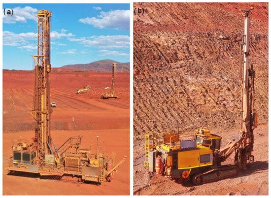
This research explores the various field observations logged, encompassing aspects such as stratigraphic unit, rock type, weathering, rock strength and GSI. The general categories for rock types include BIF, shale (SHL), detrital (DET), and the hydrated zone of alteration (HYD). Table 1 depicts the classification of weathering using a method adapted from the International Society for Rock Mechanics (ISRM) conventions [32]. In addition, Table 2 describes the ISRM strength categories for both soil and rock [33]. GSI is a rock mass classification system used to evaluate a combination of the estimated rock strength and the persistence of structures into several classes [34].

2.3. MWD Systems

MWD data collection was conducted using 22 drilling rigs. This fleet included ten Pit Viper 271 rigs by Atlas Copco (Epiroc), two Sandvik 460 rigs, two Terex SKS 12 rigs and one Bucyrus SKS 13 rig, which were used for drilling production blast holes of 0.229 m in diameter (Figure 1a). Furthermore, a Cubex QXR 920 rig, a Sandvik 560 rig, and five Atlas Copco (Epiroc) D65 drill rigs were employed for creating 0.165 m wall control blast holes (Figure 1b). The height of the benches in the iron-ore pits under study varied between 8 and 12 m. The rigs completed a sub-drill below the target pattern elevation of 2 m. The blast holes were arranged in a structured drilling pattern. Production holes followed an 8 m by 7 m grid pattern, while wall control holes had closer spacing to maintain slope stability. This spacing was designed to optimize fragmentation and minimize overbreak.

Multiple drilling variables were recorded by the MWD system, including the penetration rate (rop; m/s), the torque (tor; Nm), the force on bit (fob; kgf, the bit air pressure, (bap; kgf/cm²), and rotations per minute (rpm). The rpm data were available for only about a quarter of the sample points due to inconsistencies in the onboard sensor. As a result, they were excluded from the investigated drilling measurements. Both manually operated rigs and semi-autonomous drills collected MWD data at approximately 0.1 m intervals along the depth of each drill hole.

This study analyzed the MWD dataset from the BR pit, encompassing 75,470 blast holes with a combined depth of 844,855 m. The analysis focused on MWD data from 2 m below the hole collars to the bottom of the blast holes, as the uppermost 2 m may not reliably represent in situ rock conditions due to potential toe charge effects from the blasting of the previous bench.

MWD Feature Engineering

Multiple factors affect the accuracy of MWD data. These factors include the rock’s lithological variations and fractures, the drill rig’s management system, and external conditions, all of which may result in abnormal response values [35]. This can lead to erroneous MWD readings and potential misinterpretations of the data [36]. Consequently, the examined BR MWD dataset exhibited a relatively high noise-to-signal ratio, with no internal review of the data.

Hence, feature engineering of the MWD data in this investigation was required. To minimize the potential effect on the representation of the in situ rock due to collaring effects at the beginning of the shaft and potential blast damage from previous holes, the initial MWD dataset excluded the first 2 m of each drilling hole.

Negative drilling values caused by sensor calibration issues, temporary signal loss, or data logging errors rather than actual negative drilling responses were eliminated. Such anomalies can also occur due to sudden rig stoppages, incorrect zeroing of sensors, or transient fluctuations in the onboard MWD data acquisition system.

Linear interpolation, quartile detection techniques, and a 1.5-factor threshold were used to fill gaps in anomalous data. A Gaussian filter with a smoothing factor of 0.3 was applied to the drilling data to reduce the local effects of noise.

The interval-based data of the MWD and exploration drilling datasets were transformed into point data, incorporating geospatial coordinates along with corresponding dataset values for each data point. For exploration holes, point data were derived from downhole wireline logged desurvey data, which recorded the azimuth and dip of each hole at 10-m intervals down to the final depth. In contrast, blast hole MWD data were not desurveyed due to the production-oriented nature of the holes; instead, each point’s location was estimated by assuming a straight trajectory from the hole collar to its bottom. To fuse these datasets, the K-Nearest Neighbors (KNNs) distance-based search method was applied to match its closest MWD data point to facilitate supervised ML. The accuracy of the dataset alignment was further refined by implementing distance thresholds.

2.4. Feature Selection Algorithms

The determination of the most important features in MWD data has solely used PCA. However, this research opts for appropriate feature selection to ascertain the importance of drilling variables identified for the following geotechnical categories: rock type, weathering intensity, stratigraphic unit, Geological Strengh Index and rock strength. For this purpose, non-parametric approaches, specifically MRMR and ReliefF, were utilized on the pre-processed BR dataset. These techniques assess feature selection in different ways than making assumptions about the relationships between the variables.

MRMR, a non-parametric approach to feature selection, decouples the complex variable interactions via mutual information maximization [37]. Key features are identified by repeatedly fitting the model while alternately including and excluding each feature, then assessing the resulting performance changes. The MRMR algorithm determines the most significant MWD input by selecting the feature that contributes the greatest improvement to the model. This process is defined for categorical variables as follows:

$I (x, y) = \sum_{i, j} p (x_{i}, y_{j}) l o g \frac{p (x_{i}, y_{j})}{p (x_{i}) p (y_{j})}$

(1)

where the mutual information, I, quantifies the relationship between the two variables, x and y. This relationship is defined in the context of their joint probabilistic distribution, p(x_i,y_j), and the corresponding marginal probabilities, p(x_i) and p(y_j). Mutual information essentially provides a measure to determine a comparative level of similarity among the geotechnical classifications. In addition, the principle of minimum redundancy aims to select the outputs that are maximally dissimilar to each other. Minimal redundancy enhances the representational efficacy of the feature set with respect to the entire dataset. This not only makes the selected features a better representative of the full dataset, but it also determines the relative importance among MWD variables.

On the other hand, ReliefF is a filter-based feature selection algorithm that determines the weights of predictors for the categorical variables. Predictors that generate varying values for neighboring data points within the same class while favoring those that produce distinct values for neighbors belonging to different classes are discouraged by the algorithm [38]. The ReliefF methodology randomly samples a datapoint and then examines the impact of the neighbors of the datapoint. The technique then adjusts the weights of the drilling variables for that datapoint, with the adjustments being governed by the extent to which these features can effectively differentiate between the neighboring datapoints. The algorithm follows the logic shown below.

Assuming x_r and x_q belong to the same class, the following equation applies:

$W_{j}^{i} = W_{j}^{i - 1} - \frac{∆_{j} (x_{r}, x_{q})}{m} \times d_{r q}$

(2)

If x_r and x_q are parts of different classes, this equation applies:

$W_{j}^{i} = W_{j}^{i - 1} + \frac{p_{y_{q}}}{1 - p_{y_{r}}} \times \frac{∆_{j} (x_{r}, x_{q})}{m} \times d_{r q}$

(3)

where W_jⁱ represents the weight of predictor F_j at the i-th iteration, while p^yr and p^yq represent the prior probabilities of the classes to which x_r and x_q belong, respectively. The variable m indicates the number of iterations, Δj(x_r,x_q) measures the difference in predictor F_j between observations x_r and x_q, x_rj correspond to the values of predictor j for observation x_r, and x_q, respectively.

2.5. Classification-Based ML Methods

Different classification-based ML models were tested for their ability to classify rock types in various contexts. For example, Neural Networks (NNs), a type of machine learning model, proved effective in classifying rock types in a coal deposit in Canada [23]. However, a more specific type of NNs, known as Back Propagation NNs, failed in classifying iron-ore rock types in a United States mining operation [21]. Furthermore, two other ML techniques, Logistic Regression and Random Forests (RFs), were successful in predicting marble quality classes in Norwegian quarry [19].

In contrast to these previous studies, this research explored the following variety of ML methods: Support Vector Machines (SVMs), KNNs, Decision Trees (DTs), Naïve Bayes (NB) and Linear Discriminant Analysis (LDA). This research also employed RFs, as previous research had shown this method to be effective. Table 3 summarizes each classification-based ML method.

The predictive capacity of various classification-based ML algorithms, with computations executed on a high-performance computing system known as Pawsey Supercomputer Nimbus cloud, operating on a virtual machine with 32GB Random Access Memory and 8 virtual Central Processing Units. The MATLAB Classification Learner Toolbox was utilized to create models and evaluate prediction performance for each classification-based ML method, using key hyperparameters without optimization [45]. The available data were portioned into two sets, with 80% dedicated to training the models, and the remaining 20% used for evaluating their predictions. Tenfold cross-validation was used to evaluate the strength of the models’ predictions on the training data.

The effectiveness of the various models was compared using three specific measures: Accuracy, Overall Misclassification Cost (OMC), and Training Duration (TD).

i.: Accuracy—this measure indicates the proportion of successful predictions made by the classification model. It is determined by dividing the number of correct predictions by the total number of predictions made.
ii.: OMC—this is the total cost accumulated from incorrect predictions made by the model, computed by combining the cost matrix of misclassification with the corresponding confusion matrix.
iii.: TD—this denotes the length of time it takes for the model to complete training phase.

The criteria for these metrics are defined as follows:

$A c c u r a c y = \frac{T N + T P}{T N + F N + T P + F P}$

(4)

where TN (True Negatives) represents instances correctly identified as not belonging to the class, while TP (True Positives) refers to instances accurately classified as part of the positive class. Conversely, FP (False Positives) denotes incorrect classifications where non-class instances are mistakenly labeled as positive, and FN (False Negatives) represents cases where positive instances are incorrectly predicted as negative.

The OMC is determined, as follows:

$O M C = ({C o s t M}_{i} * {C o n f M}_{i})$

(5)

where CostM_i is the misclassification cost matrix and ConfM_i is the confusion matrix for the respective model.

4. Discussion

This study highlights the effectiveness of classification-based machine learning techniques in predicting geotechnical property classes from MWD data. By leveraging these methods, rock mechanics characterization is significantly enhanced, exceeding an order of magnitude improvement with resource development drilling techniques. While this study focused on five geotechnical data categories—stratigraphic unit, rock or soil strength, rock type, GSI, and weathering properties—it has the potential to be expanded to other categorical orebody knowledge datasets. For example, higher resolution understandings of grade, trace contaminants, alteration intensity and mineralogy, as well as other rock mass classifications systems, including rock mass rating, rock quality designation, or Q, will greatly reduce the uncertainty resulting in increased mining confidence.

This study departs from prior research by demonstrating the balanced influence of the four MWD variables. Earlier research emphasized rop and tor, utilizing PCA to determine the most important MWD measurements for rock type identification [13,16,18,21,23,47]. In contrast, both the MRMR and ReliefF feature selection methods offer invaluable insights, yet their results can diverge based on their underlying methodologies. While MRMR highlighted the significance of the bap feature, ReliefF favored towards the rop feature. Such disparities emphasize the necessity of a comprehensive approach when selecting features, considering the inherent biases and strengths of each method. Future research might explore consensus-based approaches or further investigate the specific contexts where one method may be more appropriate than the other. However, both methods revealed a relatively balanced relationship between MWD measurements in which no features were identified as having zero or minimal influence.

This study also evaluated the performance of models in predicting geotechnical categorical properties. The selection of the machine learning analytical model significantly influenced prediction results. This was evident through improved validation and testing accuracy, reduced training time, and lower validation and testing OMCs. DTs, LDA, and NB performed the weakest across the five geotechnical datasets while KNN and RFs displayed the strongest results, consistently above 90% for validation and testing accuracy for correct class identifications. Furthermore, KNN was quicker to train than RFs. For example, KNN, at 3 s, was over 20 times faster than RFs, at 64 s, for rock type. These results indicate that KNN is both the strongest and most computationally efficient model to predict geotechnical classification properties.

While this study focuses on conventional ML approaches due to their interpretability and practical application in mining operations, future research may explore deep learning methods to enhance classification performance. While these models can capture complex, nonlinear relationships in datasets, which may further refine the classification accuracy, deep learning models often function as “black boxes,” limiting their practical use in mining operations where explainability is critical. Therefore, while deep learning approaches hold potential, the trade-off between accuracy and interpretability remains a key consideration for real-time geotechnical decision-making.

However, a great deal of the variances in accuracy and training duration can be traced to differences in class distributions between the five categories (Figure 5). Rock type and stratigraphic unit had balanced distributions while the remaining categories were skewed to one class. The impact of this is observable in the consistently above 80% accuracies for GSI, rock or soil strength and weathering prediction performance results. On the other hand, the rock type and stratigraphic unit had a wider spread of accuracies, from 32% to 97%, depending on the ML algorithm. Moreover, similar physical properties may cause misclassification. For example, regarding rock type, SHL was observed to be misclassified as BIF and DET, because of its material strength lying between the relatively stronger BIF and weaker DET.

This study assumes that MWD data are of sufficient quality and reliability for geotechnical classification, with sensor calibration and data preprocessing adequately mitigating noise and inconsistencies. The approach is most applicable to structured iron ore deposits with well-characterized geological formations, and additional validation may be required for different lithologies. Furthermore, MRMR and ReliefF identified the most influential MWD variables, but their importance may vary based on site-specific conditions.

This machine learning approach is intended to complement, rather than replace, traditional geotechnical testing, which remains essential for geotechnical validation and compliance. While the models can improve spatial resolution and provide real-time insights, they should be used in conjunction with conventional methods, such as laboratory strength tests, geophysical wireline logging, and geological mapping. Ensuring a balanced approach between the AI-driven insights and field validation is crucial for robust geotechnical characterization. Model interpretation should be in conjunction with traditional geotechnical assessments to ensure a comprehensive understanding of subsurface conditions.

This study demonstrated the success of a classification-based ML technique for geotechnical classification problems but also supports the valuable role of subject matter expert oversight in complementing ML studies regarding instances of misclassification, especially concerning materials with close or overlapping properties.

5. Conclusions

The application of classification-based ML techniques in conjunction with innovative datasets, such as MWD data, has introduced fresh opportunities in the field of rock mechanics characterization. This work provides evidence for the efficacy of ML techniques in estimating geotechnical conditions. Additionally, it highlights the improvements in the characterization of rock mechanics properties beyond the scale achieved by the traditional resource development methods. The MRMR and ReliefF feature selection methods support a balanced integration of the drilling features in multivariate analysis instead of depending solely on a single feature.

Moreover, a comprehensive assessment of diverse machine learning models yielded intricate observations regarding their predictive capabilities. The KNN and RFs algorithms demonstrated a superior performance, routinely obtaining validation, and with testing accuracies exceeding 90%. The short training duration for KNN compared with that of RFs highlights its remarkable computational efficiency. Nevertheless, it is important to acknowledge that these results are closely linked to the underlying data distributions within the geotechnical classifications.

The balanced distributions of classes in the rock type and stratigraphic unit were in stark contrast to the other categories that exhibited a predominant skew towards a single class. This contrast was evident in the wide range of accuracies depending on the ML algorithm chosen in rock type and stratigraphic unit. Furthermore, the need for further examination arises from the misidentification of related materials, such as the SHL with both BIF and DET. Future work should also include other Feature Importance algorithms, such as Shapley Values, that reveal the “black box” characteristics of ML techniques to improve explainability [48,49]. Although this study focused on five geotechnical data categories, its findings establish a strong foundation for applying these methods to other categorical datasets related to orebody knowledge.

Source link

Daniel Goldstein www.mdpi.com

Greenberg News

A Machine Learning Classification Approach to Geotechnical Characterization Using Measure-While-Drilling Data

1. Introduction

2. Methods

2.1. Geological Setting

2.2. Geotechnical Field Observation Categories

2.3. MWD Systems

MWD Feature Engineering

2.4. Feature Selection Algorithms

2.5. Classification-Based ML Methods

4. Discussion

5. Conclusions

Greenberg

1. Introduction

2. Methods

2.1. Geological Setting

2.2. Geotechnical Field Observation Categories

2.3. MWD Systems

MWD Feature Engineering

2.4. Feature Selection Algorithms

2.5. Classification-Based ML Methods

4. Discussion

5. Conclusions

Related Posts

Nutrients, Vol. 17, Pages 2230: High-Fat Diet with Normal Caloric Intake Elevates TMA and TMAO Production and Reduces Microbial Diversity in Rats

The True Cost of Fast Fashion: Why Going Green Matters

Metabolites, Vol. 15, Pages 455: Effects of Eight Weeks of Aerobic Training Combined with Carbohydrate Mouth Rinse on Body Composition and Exercise Performance in Adult Men with Obesity: Evidence from Korea

Greenberg