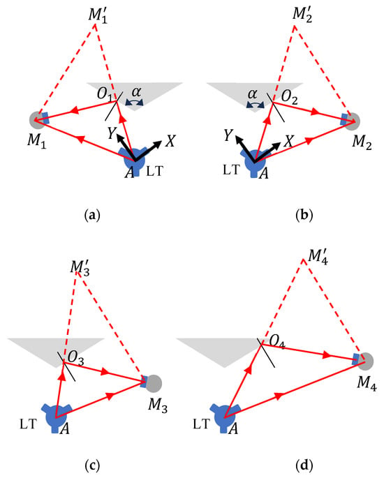
A Method to Calibrate Angular Positioning Errors Using a Laser Tracker and a Plane Mirror

We considered a plane mirror mounted on the rotation stage, as shown in Figure 3a, with the LT at

A

. In the figure, the normal vector to the mirror (solid black rectangle in the figure) is along the 0° encoder position of the rotation stage. A stationary nest is located at

M_{1}

. We performed two measurements at this position—one was a direct measurement of SMR at

M_{1}

and the other was an indirect measurement of the same SMR, i.e., after reflecting off the mirror on the rotation stage. In the LT coordinate system, the second measurement appeared to be at

M_{1}^{'}

. We then rotated the table to the next angular position, moved the stationary nest, and repeated the previous steps. Measurements at the three remaining angular positions, 22.5°, 45°, and 67.5°, are shown in Figure 3b–d.

The advantage of this approach was that there were no restrictions on the placement of the plane mirror on the table or for the alignment of the plane of rotation with respect to the LT. Further, the laser could strike the mirror at any point on the surface (assuming the mirror is flat to a level that it does not affect angle measurements), as mentioned earlier in Section 2, so there were no burdensome alignment or setup restrictions. However, because the LT laser must bounce off the mirror, the angular range that can be measured from a single LT station was limited by the angle of incidence on the mirror (theoretically ±90°, but practically less than about ±50°). Thus, multiple LT stations were required to cover the full 360°. There are two ways to tie data together from the multiple LT stations, stitching and registration, and that affected how we processed the data. These are discussed next.

2.2.1. Stitching

Figure 4 shows the measurement of angular positioning errors of a rotation stage in steps of 22.5° from six stations of the LT,

A - F

. The commanded angles of the rotation stage are given by:

$θ_{i} = (i - 1) \frac{2 π}{16},$

(4)

where i is the angular position index. While 16 positions covered the full circle (when measurements were made in increments of 22.5°), we measured errors at 17 positions so that we had an overlapping position (at 0°) to assess closure errors.

Measurements were performed from LT station $A$ for angular positions (i.e., mirror normal vector pointing along) 0°, 22.5°, 45°, and 67.5°, as described earlier. When the LT was moved to the next station, measurements were repeated at the last angular step of the previous LT station; thus, measurements from LT station $B$ were performed for angular positions 67.5°, 90°, 112.5°, and 135°. For the final LT station, $F$ , measurements were performed for angular positions 337.5° and 0°.

From the data acquired with the LT at station

A

, we calculated the unit normal vectors

\vec{n_{1, A}}, \vec{n_{2, A}}, \vec{n_{3, A}}, a n d \vec{n_{4, A}}

at angular positions 0°, 22.5°, 45°, and 67.5°, respectively. Subscript

A

indicates that the measurements were made from LT station

A

. It is unlikely that the mirror was positioned in such a manner that the normal vector to the mirror was parallel to the plane of rotation. We must, therefore, project these normal vectors to the plane of rotation before calculating angles. However, unlike in the direct approach case, we did not have data in the form of SMR centers to fit a least-squares plane. However, if we visualize the normal vectors so that one end is coincident, the vectors lie on the surface of a cone (assuming the tilt errors of the rotation stage are negligible) so that the other end lies on a circle (see Figure 5a). We could, therefore, fit a least-squares plane to these end points and project the normal vectors to that plane (see Figure 5b). This idea is also applicable to the direct approach case but we did not apply it there because we had SMR centers over the full circle that we could more easily use to find the plane. We normalized the vectors after projection and calculated the angles for position i = 1–4 with respect to 1. We let the unit normal vectors after projection to the plane of rotation corresponding to angular positions 0°, 22.5°, 45°, and 67.5° be represented using the same variables for convenience, i.e.,

\vec{n_{1, A}}, \vec{n_{2, A}}, \vec{n_{3, A}}, a n d \vec{n_{4, A}},

respectively. We will not be referring to the normal vectors prior to projection in subsequent discussions in this section; therefore, there is not a need to create a new variable.

The angles and errors are then given by:

$α_{i, A} = \cos^{- 1} (\vec{n_{i, A}} . \vec{n_{1, A}}), i = 1 t o 4$

(5)

$e_{i} = e_{i, A} = θ_{i} - α_{i, A}, i = 1 t o 4$

(6)

From the data acquired with the LT at station

B

, we calculated the unit normal vectors

\vec{n_{4, B}}, \vec{n_{5, B}}, \vec{n_{6, B}}, a n d \vec{n_{7, B}},

corresponding to angular positions 67.5°, 90°, 112.5°, and 135°, respectively. We fit a least-squares plane, projected the normal vectors to that plane, and normalized the vectors. We calculated the angles and the errors for position i = 5–7 with respect to 4 (corresponding to the 67.5° angular position):

$α_{i, B} = \cos^{- 1} (\vec{n_{i, B}} . \vec{n_{4, B}})$

(7)

$e_{i, B} = {{(θ}_{i} - θ_{4}) - α_{i, B} = θ}_{i - 4} - α_{i, B}, i = 5 t o 7$

(8)

Note that in Equation (8), the commanded angle for positions 5, 6, and 7 must be determined with respect to position 4, hence the term

{(θ}_{i} - θ_{4}),

which is equivalent to

θ_{i - 4}

. The error with respect to the first position of the LT station

A

was then obtained by summing the error of the last position of the previous station:

$e_{i} = e_{i, B} + e_{4, A}, i = 5 t o 7$

(9)

We repeated this process for the remaining LT stations, yielding the following equations:

$α_{i, C} = \cos^{- 1} (\vec{n_{i, C}} . \vec{n_{7, C}})$

(10)

$e_{i, C} = θ_{i - 7} - α_{i, C}, i = 8 t o 10$

(11)

$e_{i} = e_{i, C} + e_{4, A} + e_{7, B}, i = 8 t o 10$

(12)

$α_{i, D} = \cos^{- 1} (\vec{n_{i, D}} . \vec{n_{10, D}})$

(13)

$e_{i, D} = θ_{i - 10} - α_{i, D}, i = 11 t o 13$

(14)

$e_{i} = e_{i, D} + e_{4, A} + e_{7, B} + e_{10, C}, i = 11 t o 13$

(15)

$α_{i, E} = \cos^{- 1} (\vec{n_{i, E}} . \vec{n_{13, E}})$

(16)

$e_{i, E} = θ_{i - 13} - α_{i, E}, i = 14 t o 16$

(17)

$e_{i} = e_{i, E} + e_{4, A} + e_{7, B} + e_{10, C} + e_{13, D}, i = 14 t o 16$

(18)

$α_{i, F} = \cos^{- 1} (\vec{n_{i, F}} . \vec{n_{16, F}})$

(19)

$e_{i, F} = θ_{i - 16} - α_{i, F}, i = 17$

(20)

$e_{i} = e_{i, F} + e_{4, A} + e_{7, B} + e_{10, C} + e_{13, D} + e_{16, E}, i = 17$

(21)

2.2.2. Registration

With the LT at station $A$ , we measured the SMR nests at each of the four angular positions, 0°, 22.5°, 45°, and 67.5°. We calculated the corresponding unit normal vectors $\vec{n_{1, A}}, \vec{n_{2, A}}, \vec{n_{3, A}}, a n d \vec{n_{4, A}}$ . We also measured the six registration nests, $R_{1} - R_{6}$ . While three nests were sufficient, choosing a larger number of nests helped to minimize the effect of LT errors in the registration process. Our choice of six nests was dictated by the stands and SMRs we had available for use.

We moved the LT to station $B$ and measured the SMR nests at each of the four angular positions—67.5°, 90°, 112.5°, and 135°. We calculated the corresponding unit normal vectors $\vec{n_{4, B}}, \vec{n_{5, B}}, \vec{n_{6, B}}, a n d \vec{n_{7, B}} .$ We measured the six registration nests and calculated the matrix to transform the data acquired from LT station $B$ to $A$ . Using this matrix, we transformed the normal vectors to the frame of the LT at station $A$ . Let the resulting normal vectors be $\vec{n_{4, B, A}}, \vec{n_{5, B, A}}, \vec{n_{6, B, A}}, a n d \vec{n_{7, B, A}}$ , where the subscript $B$ indicates that the data were acquired from station $B$ and the subscript $A$ indicates that the data had since been transformed to station $A$ . We repeated this process for the other LT stations and calculated the normal vectors.

As we noted earlier, it is unlikely that the mirror was positioned in such a manner that the normal vectors to the mirror were parallel to the plane of rotation. We projected these normal vectors to the plane of rotation, as described in Section 2.2.1, normalized them, and calculated angles with respect to the 0° position. Note that in this case, we collected the normal vectors from all the LT positions, transformed them to LT station A, and then fit a single plane. In the case of stitching, we had to perform this operation for each LT station. Also, as in Section 2.2.1, we used the same variables for the normal vectors after projection to the plane for convenience. We will henceforth not be referring to the normal vectors prior to projection in this section.

The angles are given by:

$α_{i} = \cos^{- 1} (\vec{n_{i, A}} . \vec{n_{1, A}}), i = 1 t o 4$

(22)

$α_{i} = \cos^{- 1} (\vec{n_{i, B, A}} . \vec{n_{1, A}}), i = 4 t o 7$

(23)

$α_{i} = \cos^{- 1} (\vec{n_{i, C, A}} . \vec{n_{1, A}}), i = 7 t o 10$

(24)

$α_{i} = \cos^{- 1} (\vec{n_{i, D, A}} . \vec{n_{1, A}}), i = 10 t o 13$

(25)

$α_{i} = \cos^{- 1} (\vec{n_{i, E, A}} . \vec{n_{1, A}}), i = 13 t o 16$

(26)

$α_{i} = \cos^{- 1} (\vec{n_{i, F, A}} . \vec{n_{1, A}}), i = 16 t o 17$

(27)

We then calculated the errors in the angles:

$e_{i} = θ_{i} - α_{i}, i = 1 t o 17$

(28)

Because we measured some angular steps twice, i.e., as the last measurement from a given LT station and as the first measurement from the next LT station, we had repeat measurements for those positions. These repeat measurements are not required for the registration approach but are required for the stitching approach.

Source link

Bala Muralikrishnan www.mdpi.com

Greenberg News

A Method to Calibrate Angular Positioning Errors Using a Laser Tracker and a Plane Mirror

2.2.1. Stitching

2.2.2. Registration

Greenberg

2.2.1. Stitching

2.2.2. Registration

Related Posts

NOAA Office for Coastal Management

Development and Performance Study of Continuous Oil–Water Separation Device Based on Superhydrophobic/Oleophilic Mesh

Novel Buccal Xanthan Gum–Hyaluronic Acid Eutectogels with Dual Anti-Inflammatory and Antimicrobial Properties

Greenberg