3.1. MSGA Model for a Finite Slope
The water exchange among the slope consists of the recharge from the rainfall infiltration and the discharge of the seepage parallel to the slope surface. For the infinite slope, since the volume of the recharge from the infiltration of rainwater is much greater than the discharge of the seepage parallel to the slope surface, it is reasonable to neglect the influence of seepage parallel to the slope surface. However, the seepage parallel to the slope surface should be considered for the finite slope. Few expansions of the GA model have considered both the existence of the transition layer and the seepage parallel to the slope surface for the finite slope. Therefore, the MSGA model is proposed. While soil parameters are widely recognized to exhibit spatial variability, most of the modified GA models assume that soil is homogeneous for simplicity [
19,
28,
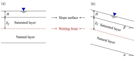
29]. The MSGA model assumes that soil is homogeneous. The MSGA model considers the seepage parallel to the slope based on the SGA model. The schematic diagram of the MSGA model for a finite slope during a rainfall event is shown in
Figure 4. Usually, the ponding water head is small compared to the suction head of the wetting front, so the value of the ponding water head is assumed to be equal to 0 m.
The infiltration process during intense rainfall can be divided into two stages depending on the relation between rainfall intensity and infiltration capacity. At stage 1, the rainfall intensity is less than the infiltration capacity. At stage 2, the rainfall intensity is greater than the infiltration capacity. The infiltration ability of the slope can be expressed as follows:
where ia denotes infiltration ability (m/h).
Since the permeability coefficient has an exponential relation to the water content, the permeability coefficient in the saturated state is much greater than that in the unsaturated state. Therefore, the MSGA model only considers the seepage in the saturated layer at stage 2.
At stage 1, which represents the initial stage of the rainfall infiltration, the shallow soil of the slope is unsaturated. Rainwater infiltrates into the soil entirely because the infiltration capacity is greater than the rainfall intensity. Therefore, the infiltration rate is dependent on the rainfall intensity, which can be calculated by:
in which q denotes the rainfall intensity (m/h).
With the infiltration of rainwater, the state of shallow soil changes from unsaturated to saturated. When the wetting front forms, this is called the critical time. The infiltration ability (
ia) is equal to the projection of the rainfall intensity on the slope surface (
qcosβ) at the critical time. At this time, the depth of the wetting front can be calculated by combing Equations (6) and (7), which is expressed as follows:
where Zfc is the depth of the wetting front at the critical time (cm). Based on Equations (2) and (3), the cumulative infiltration depth is defined by:
where I is the cumulative infiltration depth (m). The cumulative infiltration depth at the critical time and the critical time can be calculated as follows:
where Ic is the cumulative infiltration depth at the critical time (m), and tc is the critical time (h).
Stage 1 changes to stage 2 when the critical time is reached. At stage 2, the shallow soil is saturated. The moving speed of the wetting front is controlled by the rainfall infiltration and the seepage parallel to the slope surface. The effect of the rainfall infiltration on the moving speed of the wetting front can be expressed as follows:
According to the law of conservation of mass and Darcy’s law, the following equation can be obtained:
where L is the length of the surface for the finite slope (m). Therefore, the effect of the seepage on the moving speed of the wetting front can be expressed as follows:
The actual infiltration speed of the wetting front is calculated by combining Equations (12) and (14), which is expressed as follows:
Since the expression for Zf obtained by integrating Equation (15) is complicated, it is suggested to use the numerical method to calculate Zf. The depth of the wetting front at stage 2 is calculated by the Runge-Kutta 4th-order method, with the initial condition that Zf = Zfc and t = tc.
3.2. Stability Analysis for Various Sliding Surfaces
Slope failure induced by rainfall frequently occurs, and the shallow failure is always parallel to the slope surface [
11,
30]. The shallow failure may occur along the wetting front or the interface between the saturated layer and the transition layer. Besides shallow failure, failure also occurs along the surface of the bedrock.
For the slip parallel to the slope surface along the wetting front, the factor of safety can be calculated by:
in which Fs denotes the factor of safety, Gs denotes the gravity of the soil in the saturated layer (N/m), Gt denotes the gravity of the soil in the transition layer (N/m), φ′ denotes the effective friction angle of the natural soil (°), φb is the angle that denotes the contribution of matrix suction against shear strength (°), c′ denotes the effective cohesion of the natural soil (Pa), ua denotes pore air pressure (Pa), uw denotes pore water pressure (Pa), and P denotes the seepage force (N/m).
According to Vanapalli [
31], tan
φb can be expressed as follows:
in which Θ = (θ − θr)/(θs − θr) denotes relative water content. For the slip parallel to the slope surface along the wetting front, combing Equations (16) and (17), the factor of safety can be calculated by:
in which Θi = (θi − θr)/(θs − θr).
For the slip parallel to the slope surface along the interface between the transition layer and saturated layer, the factor of safety can be calculated by:
in which φs′ represents the effective friction angle of the saturated soil (°), and cs′ represents the effective cohesion of the saturated soil (Pa).
For the slip along the surface of the bedrock, the factor of safety can be calculated by:
in which Gs denotes the gravity of the soil in the natural layer (N/m).
3.3. Variation in Fs for a Natural Slope during a Rainfall Event
Natural slopes usually have irregularly curved surfaces and slip surfaces, which makes it difficult to calculate the depth of the wetting front for natural slopes during intense rainfall. Without the depth of the wetting front, the stability of the natural slope cannot be evaluated by the limit equilibrium method.
The slice method is adopted to calculate the depth of the wetting front. The sides of the slices are vertical. The curved slope surface and slip surface of each slice are replaced by straight lines. Each slice can be deemed as a finite slope. The simplified model of the natural slope is shown in
Figure 5. Then, the MSGA model is used to calculate the depth of the wetting front of each slice.
According to Equation (15), the depth of the wetting front during intense rainfall is influenced by the slice’s dip angle and the slice’s length. Therefore, different slices have different depths of the wetting front. The depth of the wetting front should be continuous. This kind of discontinuity can be reduced by increasing the number of slices.
A slice is divided into three layers based on the MSGA model, which is shown in
Figure 6a. The gravity of the
ith slice can be expressed as follows:
where Gi represents the gravity of the ith slice. Gis represents the gravity of the saturated layer of the ith slice (N/m), Git represents the gravity of the transitional layer of the ith slice (N/m), and Gin represents the gravity of the natural layer of the ith slice (N/m). γs represents the unit weight of the saturated soils (N/m3), and γi represents the unit weight of the natural soils (N/m3). Ais represents the area of the saturated layer of the ith slice (m2), and Ain represents the area of the natural layer of the ith slice (m2).
According to Yao [
20],
Git can be expressed as follows:
where Li denotes the length of the slope surface of the ith slice (m), βi denotes the dip angle of the slope surface of the ith slice (°), and αi denotes the dip angle of the slip surface of the ith slice (°).
In the saturated layer, the seepage parallel to the slope surface would cause the seepage force parallel to the slope surface, which is expressed as follows:
where Pi is the seepage force of the ith slice (N/m), and γw is the unit weight of water (N/m3). The force diagram of the ith soil slice is shown in Figure 6b.
The factor of safety can be calculated by:
where Fs represents the factor of safety, Ei represents the thrust between the ith slice and the (i + 1)th slice (N/m), and li represents the length of the slip surface (m). Equation (24) can be written as follows:
To be consistent with reality, it is assumed that there is no tensile stress between adjacent slices. Therefore, the value of
Ei is replaced by 0 when the calculation result of
Ei is smaller than 0, which can be expressed as follows:
The process for calculating the stability of the natural slope is illustrated as follows: Firstly, an arbitrarily small value of
Fs is input. Then, for
i = 1 to
i = n, the values of
Ei can be calculated in sequence. If
En is not equal to 0, then
Fs will be reset with a greater value, and the value of
Ei will also be recalculated.
Fs needs to be iterated until
En equals 0. When
En equals 0, the corresponding
Fs is the actual factor of safety of the slope. The process of the proposed method is shown in
Figure 7.