A Simulation Study on Pressure Control in Oil Well Drilling Using Gain-Scheduled PID Controllers

1. Introduction

The growing demand for oil and gas for energy production has driven exploration into increasingly challenging and hostile environments, such as the drilling of complex wells in deep waters and offshore platforms. Despite advances in other forms of energy, fossil fuel extraction remains a fundamental industry, with global investments in its exploration amounting to hundreds of billions of USD annually [1].

Oil field exploration for primary extraction involves three main stages: prospecting, drilling, and extraction. Prospecting includes locating sedimentary basins through detailed analysis of the soil and subsoil. After identifying a potential oil reserve, drilling begins to establish a connection between the underground deposits and the surface, commonly known as a drilling well. Initial success in this phase can lead to additional drilling to assess the extent of the reservoir and determine the viability of extraction. Finally, the extraction stage involves bringing fossil fuels to the surface [2].

Drilling is generally the most costly, complicated, and dangerous phase of oil exploration. This process involves the application of a force to a set of equipment, including a metal tower and a drill string with a drill bit at its end. This drill string is composed of pipes between 9 and 27 m long, connected to each other and added as drilling progresses [3]. During this phase, there is a significant risk of catastrophic incidents that can cause economic losses, environmental damage, and, in extreme cases, loss of human life. Tragic examples include the accidents on the Enchova Platform (Campos Basin, RJ, Brazil) in 1984 and 1988 and the explosion on the Piper Alpha platform in the North Sea in 1988, which resulted in multiple fatalities and significant financial losses [4].

To prevent explosions and control gas or fluid influx (high underground pressure during drilling), it is crucial to apply advanced process control technologies. This not only minimizes associated risks but also optimizes production costs in hydrocarbon extraction. A critical factor during drilling is the control of bottom-hole pressure (BHP) [5]. In conventional drilling operations, the common response to an unexpected influx is to activate blowout preventers, key devices that connect the wellhead at the seafloor to the platform, shutting in the well and, in many cases, abruptly stopping all equipment. Modern drilling technology, known as Managed Pressure Drilling (MPD), introduces a pressure control technique that adds an additional layer of controlled pressure, on top of hydrodynamic and hydrostatic pressures, using a choke valve [6].

On offshore platforms, operators manually adjust the valve actuators during MPD operations. However, due to rapid pressure fluctuations, closing the valve to reduce bottom pressure, if excessive, presents a significant challenge. Manual drilling operations have a high potential for error and present response time limitations. Therefore, implementing automated control systems to maintain the desired bottom-hole pressure is necessary [7].

The integration of digital and automation technologies is emerging as a key component in the oil and gas industry, enabling improved operational efficiency and reducing risks associated with drilling. Digitalization has driven the adoption of technologies such as artificial intelligence, the Internet of Things (IoT), and process automation, which are transforming the way operations are managed on offshore platforms. These advancements are essential for achieving sustainability goals and improving safety in operations, aligning with the energy transition toward a net-zero future by 2050 [8].

Despite these advances, there is a clear gap in the literature regarding the integration of PID controllers adjusted by Gain Scheduling (GS) to handle the complexity of nonlinear systems in drilling at different operational depths [9]. While PID controllers are known for their simplicity and effectiveness in many industrial systems, their application in systems with nonlinear behavior, such as drilling wells, presents significant challenges due to the lack of dynamic adaptation to the variable conditions of the process. By applying GS, the PID gains are adjusted in real time according to operating conditions, providing a more manageable and less costly solution to tackle the system’s complexity and improve the maneuverability and stability of the drilling process [10].

In the context of BHP control, initial studies such as Kaasa (2006) developed mathematical models that describe the drilling process and bottom-hole pressure based on surface measurements. These models allow the representation of the drilling system considering the fluid movement within the drill string [11]. Various authors have used this approach to design controllers and test them through simulations of typical problems in drilling, such as circulation losses, power failures, and influxes [12].

The proposed Gain-Scheduled PID control method introduces significant improvements in stability and robustness for oil well drilling systems compared to traditional control strategies. Unlike conventional PID controllers, which require manual tuning, the Gain-Scheduled approach automatically adapts to varying drilling depths, ensuring consistent performance. Additionally, this method outperforms Model Reference Adaptive Control (MRAC) by providing enhanced stability at deeper operational points while maintaining ease of implementation and computational efficiency. These advantages position the proposed method as a practical and innovative solution to address the challenges of nonlinear system dynamics in drilling operations.

However, due to the inherent complexity of the problem and the need to control pressure at different operational points, such as various drilling depths, specific adjustments of control parameters are required [13]. To tackle this challenge, an Internal Model Control (IMC) strategy with two degrees of freedom is proposed for tuning and specifying PID parameters. In parallel, the behavior of these parameters was evaluated through simulations using the Gain-Scheduled (GS) method in Simulink/Matlab. Additionally, an Adaptive Controller based on a reference model was implemented to analyze system responses and compare the results obtained. This comparative analysis aimed to identify the methodology that offers superior performance in terms of stability, robustness, ease of implementation, and programming.

The remainder of this paper is organized as follows: Section 2 presents the mathematical modeling of the drilling system, including nonlinear equations, linearization, and the Laplace representation. Section 3 details the design of the PID controller parameters using the IMC methodology and their application across various depths. Section 4 discusses the implementation and comparison of two adaptive controllers: the Gain-Scheduled PID and Model Reference Adaptive Control (MRAC). This section also includes the simulation results for different operational scenarios. Finally, Section 5 concludes the study by summarizing the key findings, emphasizing the advantages of the proposed control method, and suggesting directions for future research.

2. Wellbore Pressure Model

This section presents mathematical models based on fluid mechanics, using the equation of state and Reynolds transport equations (continuity and momentum). These models allow the derivation of differential equations that describe the bottom-hole pressure and flow through the control valve. The model, originally proposed by Kassa (2006) and used by [12,13,14,15,16], serves as the basis for further analysis. 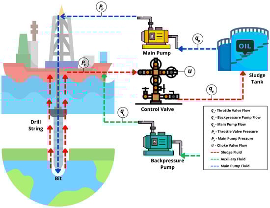Figure 1 shows a typical schematic of a well drilling system.

In this system, the main pump extracts fluid (q_p) from the sludge tank. The drilling fluid (mud) then travels through the pipes (P_p) to the drill string and the bit, ascending through the annular region while carrying rock debris from the drilling to the well’s exit (P_e). The drill string is assembled by adding pipes as the drilling depth increases. Subsequently, the fluid passes through the choke valve (u), where effective control measures optimally regulate the pressure at the drill bit. Finally, the fluid returns to the initial sludge tank (q_e), facilitating fluid mixing. In situations requiring higher pressure, a backpressure pump (q_c) can be added [16,17,18,19].

2.1. Linearization of Bottom-Hole Pressure Dynamics

To implement the Internal Model Control method, it was necessary to model the process as a set of linear equations. Linearizing nonlinear models is a common, crucial, and beneficial practice in engineering. This linearization process involves expanding the nonlinear function into a Taylor series around the operating point, retaining only the linear term [14].

The Kassa model is presented in (1)–(4):

$V_{d} {\dot{P}}_{p} = β_{d} (q_{p} - q_{b}),$

(1)

$V_{a} {\dot{P}}_{e} = β_{a} (q_{b} + q_{r} + q_{c} - q_{e}),$

(2)

$\begin{matrix} {\dot{q}}_{b} M & = & P_{p} - P_{e} - F_{a} (q_{b} + q_{r})^{2} - F_{d} {q_{b}}^{2} + (ρ_{d} - ρ_{a}) g h_{b} \end{matrix},$

(3)

$\begin{matrix} P_{b} M & = & \begin{matrix} M_{d} P_{e} + M_{a} P_{p} + M_{d} F_{a} (q_{b} + q_{r})^{2} - M_{a} F_{d} {q_{b}}^{2} + (M_{a} ρ_{d} - M_{d} ρ_{a}) g h_{b} \end{matrix} \end{matrix} .$

(4)

First, the input and output variables of the system, represented by the previously mentioned nonlinear equations, had to be identified. The input variables were those that could be manipulated to influence other variables, such as the parameters q_p, q_r, q_d, q_e, and h_b in this case.

Using Equations (1)–(4), the Taylor series expansion was applied, resulting in equations that were then arranged into the state equation of the dynamic system, as shown in Equations (5)–(8).

$J_{a} = (\begin{matrix} \frac{\partial \dot{P_{p}}}{\partial P_{p}} & \frac{\partial \dot{P_{p}}}{\partial P_{e}} & \frac{\partial \dot{P_{p}}}{\partial q_{b}} \\ \frac{\partial \dot{P_{e}}}{\partial P_{p}} & \frac{\partial \dot{P_{e}}}{\partial P_{e}} & \frac{\partial \dot{P_{e}}}{\partial q_{b}} \\ \frac{\partial \dot{q_{b}}}{\partial P_{p}} & \frac{\partial \dot{q_{b}}}{\partial P_{e}} & \frac{\partial \dot{q_{b}}}{\partial q_{b}} \end{matrix}),$

(5)

$J_{b} = (\begin{matrix} \frac{\partial \dot{P_{p}}}{\partial q_{p}} & \frac{\partial \dot{P_{p}}}{\partial u} & \begin{matrix} \frac{\partial \dot{P_{p}}}{\partial q_{r}} & \frac{\partial \dot{P_{p}}}{\partial h_{b}} \end{matrix} \\ \frac{\partial \dot{P_{e}}}{\partial q_{p}} & \frac{\partial \dot{P_{e}}}{\partial u} & \begin{matrix} \frac{\partial \dot{P_{e}}}{\partial q_{r}} & \frac{\partial \dot{P_{e}}}{\partial h_{b}} \end{matrix} \\ \frac{\partial \dot{q_{b}}}{\partial q_{p}} & \frac{\partial \dot{q_{b}}}{\partial u} & \begin{matrix} \frac{\partial \dot{q_{b}}}{\partial q_{r}} & \frac{\partial \dot{q_{b}}}{\partial h_{b}} \end{matrix} \end{matrix}) .$

(6)

The input u is the sum of the flow rate from the throttling valve and the flow produced by the backpressure pump (u = q_c − q_e).

$J_{c} = (\frac{\partial P_{b}}{\partial P_{p}} ⋮ \frac{\partial P_{b}}{\partial P_{e}} ⋮ \frac{\partial P_{b}}{\partial q_{b}}),$

(7)

$J_{d} = (\frac{\partial P_{b}}{\partial q_{p}} ⋮ \frac{\partial P_{b}}{\partial u} ⋮ \frac{\partial P_{b}}{\partial q_{r}} ⋮ \frac{\partial P_{b}}{\partial h_{b}}) .$

(8)

The state equation of a dynamic system describes the relationship between the input variables (U), state variables (X), and output variables (Y).

$\dot{X} = J_{a} X + J_{b} U, x (0) = x_{o}, Y = J_{c} X + J_{d} U$

(9)

Equations (10) and (11) illustrate the arrangement of Equation (9), highlighting its identified input, output, and state variables.

$(\begin{matrix} \dot{P_{p}} \\ \dot{P_{e}} \\ \dot{q_{b}} \end{matrix}) = J_{a} (\begin{matrix} P_{p} \\ P_{e} \\ q_{b} \end{matrix}) + J_{b} (\begin{matrix} q_{p} \\ u \\ \begin{matrix} q_{r} \\ h_{b} \end{matrix} \end{matrix}), (\begin{matrix} P_{p} (0) \\ P_{e} (0) \\ q_{b} (0) \end{matrix}),$

(10)

$P_{b} = J_{c} (\begin{matrix} P_{p} \\ P_{e} \\ q_{b} \end{matrix}) + J_{d} (\begin{matrix} q_{p} \\ u \\ \begin{matrix} q_{r} \\ h_{b} \end{matrix} \end{matrix}) .$

(11)

Equations (12)–(15) present the parameters of the state equation for the linearized dynamic system.

$J_{a} = (\begin{matrix} 0 & 0 & - \frac{β_{c}}{V_{c}} \\ 0 & 0 & \frac{β_{a}}{V_{a}} \\ \frac{1}{M} & \frac{- 1}{M} & - \frac{2}{M} [(F_{c} + F_{a}) \bar{q_{b}} + F_{a} \bar{q_{r}}] \end{matrix}),$

(12)

$J_{b} = (\begin{matrix} \begin{matrix} \frac{β_{c}}{V_{c}} & 0 \end{matrix} & 0 & 0 \\ \begin{matrix} 0 & \frac{β_{a}}{V_{a}} \end{matrix} & \frac{β_{a}}{V_{a}} & 0 \\ \begin{matrix} 0 & 0 \end{matrix} & - \frac{2 F_{a}}{M} (\bar{q_{b}} + \bar{q_{r}}) & \frac{{(ρ}_{c} - ρ_{a}) g}{M} \end{matrix}),$

(13)

$J_{c} = (\frac{M_{a}}{M} ⋮ \frac{M_{c}}{M} ⋮ - \frac{2}{M} [(F_{c} M_{a} - F_{a} M_{c}) \bar{q_{b}} + F_{a} M_{c} \bar{q_{r}}]),$

(14)

$J_{d} = (0 ⋮ 0 ⋮ \frac{{2 F}_{a} M_{c}}{M} (\bar{q_{r}} + \bar{q_{b}}) ⋮ \frac{{(M_{a} ρ}_{c} - {M_{c} ρ}_{a}) g}{M}) .$

(15)

Equation (16) represents the detailed mathematical derivation of the transfer function that links the control signal u(s) to the bottom-hole pressure P_b(s) during drilling. It was derived using the Laplace transform of the system’s nonlinear equations and incorporates the system’s physical parameters and their interactions. This equation is highly complex and includes multiple terms that account for second-order dynamics and cross-parameter interactions.

$\frac{P_{b} (s)}{u (s)} = \frac{\frac{\partial P_{b}}{\partial P_{e}} \frac{\partial \dot{P_{e}}}{\partial u} s^{2} + (\frac{\partial P_{b}}{\partial q_{b}} \frac{\partial \dot{q_{b}}}{\partial P_{e}} \frac{\partial \dot{P_{e}}}{\partial u} - \frac{\partial \dot{q_{b}}}{\partial q_{b}} \frac{\partial \dot{P_{e}}}{\partial u} \frac{\partial P_{b}}{\partial P_{e}}) s + \frac{\partial P_{b}}{\partial P_{p}} \frac{\partial \dot{q_{b}}}{\partial P_{e}} \frac{\partial \dot{P_{e}}}{\partial u} \frac{\partial \dot{P_{p}}}{\partial q_{b}} - \frac{\partial \dot{q_{b}}}{\partial P_{p}} \frac{\partial \dot{P_{p}}}{\partial q_{b}} \frac{\partial \dot{P_{e}}}{\partial u} \frac{\partial P_{b}}{\partial P_{e}}}{s (s^{2} - s \frac{\partial \dot{q_{b}}}{\partial q_{b}} - \frac{\partial \dot{q_{b}}}{\partial P_{p}} \frac{\partial \dot{P_{p}}}{\partial q_{b}} - \frac{\partial \dot{q_{b}}}{\partial P_{e}} \frac{\partial \dot{P_{e}}}{\partial q_{b}})},$

(16)

$\frac{P_{b} (s)}{u (s)} = \frac{K}{s (τ s + 1)},$

(17)

However, to design the IMC controller, the process had to be modeled according to a predefined structure [18]. Equation (17), on the other hand, is a simplified representation of the system, modeled as a first-order process with an integrative element. This form was chosen to facilitate the design of the Internal Model Control (IMC) controller. The parameters K (gain) and τ (time constant) were obtained by fitting the response of the detailed model (Equation (16)) to a first-order process with integration. This approximation captured the dominant behavior of the system while reducing its complexity, allowing for the straightforward application of control design techniques.

2.2. Implementation of the Process Model

To implement the process model, it was essential to have the well and reservoir parameters, which were then integrated into the model. Studies conducted by [20,21,22,23,24,25,26,27] collected data from well and reservoir sections at various depths. Table 1 presents the specifications that remain across all laboratory operating points. Values for diameter and area are added to the table for the drill string and annular regions (d_d, d_a, A_d, and A_a), while Table 2 details parameters that vary with depth, thereby altering the process model. These values were calculated following a linear trend based on the parameters reported by the aforementioned authors.

The data from Table 1 and Table 2 were integrated into Equations (12)–(15). The state equation could be represented using the Laplace transform in Equation (16). Subsequently, the process model had to be adapted to a predefined structure compatible with IMC-type control, which will be explained in the next chapter. The structure was configured in Simulink using the data from Table 1 and Table 2, and simulations were conducted using the Dormand–Prince algorithm with a sampling rate of 0.01 s. Once the process was set up, the function u(t) was excited with a step function. The response to this excitation was fitted to Equation (17) using the Curve Fitting tool in Matlab R2020a, achieving a coefficient of determination of 0.99.

Figure 2 shows the unstable response (due to the integrator term) across different operational points. It can be observed that, as the drilling depth increases, the slope of the trend decreases. This indicates that at shallower depths, the process is more sensitive to the control u(t); in other words, pressure variation occurs more rapidly at shallower depths with a given action of the control valve. The results exhibit a trend similar to that observed experimentally in [21].

3. Design of PID Parameters

The objective of this chapter is to determine the PID parameters for different operational points, which in this case correspond to drilling depths of 500, 1000, 2000, 3000, 4000, and 5000 m. To create the table with the parameters, it was necessary to find the optimal tuning. One of the most commonly used controllers in the industry for managing unstable processes (such as integrative ones) is the IMC controller. Internal Model Control, introduced by [28], features a tuning parameter related to the closed-loop response time, allowing the direct assessment of the benefits of dead time compensation. This approach offers a suitable structure that simplifies PID controller tuning, thereby enhancing the performance and robustness of the desired system [29].

In [30], a study is presented that develops an analytical method for tuning PID parameters in integrative processes with time delay based on [31], using an optimization method to determine the PID parameters that ensure greater robustness and system performance. The main difference between Jin and Liu’s method and the traditional IMC method is the incorporation of a filter in the input signal in the feedback loop. The structure of the feedback filter is defined according to Equation (18).

$f (s) = \frac{b^{2} s^{2} + c s + 1}{{(λ s + 1)}^{2} (β s + 1)}$

(18)

where $b = (2 T β λ + c L T - β λ^{2} + λ^{2} T) / (T + L)$ and $c = 2 λ + β + L$ ; the constants $λ$ and $β$ are the filter parameters that were determined through optimization in the study.

The controller achieves the desired performance for both transient response and disturbance rejection simultaneously, using two-degrees-of-freedom control, as shown in Figure 3. F(s) is an additional filter called a set-point or reference filter, due to its location in the feedback control system, which improves transient response behavior. The procedures are formulated as an optimization problem, where parameters are obtained by minimizing the performance index of load disturbance rejection represented by the integral absolute error, denoted by IAE-d [32]. Furthermore, a good controller should provide the desired level of robustness, with robustness measured by the maximum sensitivity function Ms, formulated as a constraint [33]. Although the optimization method employed may be complex, analytical tuning rules were provided for both the controller and the set-point filter (19).

$F (s) = \frac{(λ s + 1) (β s + 1)}{b^{2} s^{2} + c s + 1}$

(19)

The first-order integrative model with time delay is represented as shown in Equation (20).

$\bar{G} (s) = {\frac{K}{s (τ s + 1)} e}^{- θ s}$

(20)

Using

α = L / (L + T)

and the transformation

\hat{s} = (L + T) s

, the first-order integrating model plus time delay is represented as shown in Equation (21).

$\bar{G} (s) = \frac{K^{'}}{\hat{s} [(1 - α) \hat{s} + 1]} e^{- α \hat{s}}$

(21)

where $K^{'} = K (L + T)$ . The method in [31] uses Equation (38) as the model for controller design, with α ranging from 0.01 to 1. The relationship between λ and β is represented by Equation (22).

$ε = \frac{β}{λ} = \{\begin{matrix} 1 & , 0.01 \leq α \leq 0.35 \\ \frac{- 0.06 (α - 1)}{α^{3}} & , 0.35 < α \leq 1 \end{matrix}$

(22)

Figure 4 was used to determine the PID parameters based on the system’s robustness (Ms) and the parameter α.

The presence of time delay in Equation (20) significantly impacts the stability of the system. Time delay introduces a phase lag in the system response, which can lead to reduced performance or instability if not adequately compensated. Specifically, in drilling systems, excessive time delay can hinder the controller’s ability to react to disturbances, resulting in oscillations or even a loss of pressure control stability.

The maximum allowable time delay for the considered system model was determined by evaluating the stability margin of the system. Using the transfer function approximation in Equation (20), the Nyquist criterion was applied to analyze stability under varying time delays. It was found that the system remains stable for delays up to τ_max = 0.25 s. Beyond this threshold, the phase lag introduced by the delay leads to a violation of the stability margin, causing the system to become unstable.

4. Results

The simulation results for the IMC methodology with two degrees of freedom (IMC+2DOF) at different depths (500, 1000, 2000, 3000, 4000, and 5000 m) are presented for analysis purposes. These results detail the response of the IMC+2DOF-controlled system for various robustness levels (Ms) and depths, using a unit step input at the start, followed by a disturbance step after 100 s, as illustrated in Table 3 and Figure 5. These results present parameters related to the performance of the response, including overshoot, rise time, settling time, and the integral absolute error in the presence of disturbance (IAE-d), at each operating point [23].

The main feature of the IMC+2DOF methodology was that the transient response overshoot was zero, due to the action of the reference filter F(s), as observed in these results. Unlike other traditional IMC controllers, the system’s robustness was inversely proportional to the disturbance rejection performance index, meaning it showed better transient response performance with higher disturbance rejection. This behavior can be explained by the rise time parameter in this procedure being directly proportional to the system’s robustness, a trend also present in other controllers that lack a reference filter, resulting in damped oscillations in the transient response, extending the settling time [34]. Therefore, this behavior did not manifest with the IMC+2DOF controller because the filter caused the response to become over-damped with a significantly faster settling time.

4.1. Specification of Gain Scheduling (GS) Controller

Offshore drilling, for example, presents a much more complex dynamic compared to other petrochemical processes. The operating range can vary significantly due to factors such as increased drilling depth, which affects the control volume and pressure, variations in fluid density due to pressure increase, and the movement of waves, among others [35]. One of the main challenges in tuning PID controller parameters is that the optimal values for a specific operating condition may not be suitable for others due to inherent process variations. In practice, PID tuning is often adjusted to achieve robust performance across a wide range of operational conditions [33]. However, in certain scenarios, this tuning may amplify system disturbances.

Once the trends of the PID controller were analyzed, the parameters of the intended controller were specified using the Gain Scheduling method. The operations were simulated for each depth, and a similar value of robustness was adopted for the controllers; in this case, the value Ms = 1.8 was considered [35].

Likewise, for each depth, PID hooks were adopted that characterized the best tuning of the two parameters, thus guaranteeing the best performance of the responses, as demonstrated by the IMC+2GL methodology together with a robustness of Ms = 1.8. In detail, the two PID parameters are presented in Table 4.

4.2. GS Controller and MRAC: Implementation

This section is a comparison of the results obtained from the simulation of two adaptive controllers, using Gain Scheduling (GS) and the reference model (MRAC), both implemented considering even the delay time in the modeling of the process and tested at different operating points (or depths).

The structure of the GS controller, according to Figure 6, was implemented using the tools of the Simulink application, through the Lookup Table command, where we inserted the values of two proportional integrative and derivative hooks for different operating points, obtained according to Table 4. This command identified the system and made the values of the PID controller parameters modified and thus compensated for the change in the process, such as changes in the operating points. For this reason, it was important to fine-tune two parameters of the PID controller.

Also, for comparison and analysis purposes, the reference model adaptive controller (MRAC) based on the Lyapunov theory was used [36]. Also, due to the presence of the delay time in the system, a Smith predictor was added so that the output signal of the system was divided into the drilling system signal without the delay time and a signal with the delay time. Afterwards, we connected these two signals and fed them back to the controller.

The structure of the MRAC adaptive controller, according to Lyapunov, is presented in Figure 7, and the values of the controller parameters (γ) and the parameters of the reference model, obtained from [16], were implemented in the Simulink platform.

As already presented, in Table 4, the k_p, t_i, and t_d drills are shown for different drilling depths (500, 1000, 2000, 3000, 4000, and 5000 m). The GS controller methodology consisted of specifying all previously obtained data and storing this information in a table and using it to compensate for the instabilities of the system response. The control BMI with a filter (BMI+2GL) developed by [31] was chosen for the start of this table and used in simulations of different depths. Next, we compared the results of this simulation with the results obtained with the adaptive controller developed by [37].

4.3. GS Controller and MRAC: Simulation

During the drilling operation of oil wells, as mentioned in previous chapters, disturbances eventually arise that cause pressure fluxes. The pipe connection operation, which involves a continuous procedure when reaching greater depths is desired, can be cited as sources of disturbance. Also, drilling in geological zones with greater pressure can create influences and circulation losses, among others [2]. For the purpose of testing the performance of the GS controller proposed in this study, the responses of the oil well drilling system were evaluated by simulating real-problem situations present during operation and compared with the presented MRAC controller (Figure 8).

4.3.1. Pressure Tracking Control

The system was simulated and responses were obtained for the GS and MRAC controllers, as already specified. We evaluated the performance and behavior of the response to the follow-up of the desired pressure. The pressure levels of the drilling could be elevated and varied, so in this study a pressure range from 190 to 200 bar was considered. For the different drilling depths in the study (500, 1000, 2000, 3000, 4000, and 5000 m), a desired positive-step function that varied from 190 to 200 bars of pressure was implemented in the initial instant for 100 s. Next, the degrade function was modified to reach a negative value by returning to the initial press. The responses of the system to control the desired pressure, for the different points in the operation, are illustrated in Figure 9.

4.3.2. Power Loss

The initial chapters describe some problems that may arise during the drilling operation of an oil well, and one of them is the problem of power loss, which can be represented by the change in the value of the main pump flow rate. There is also the problem of pipe connection, which converges with the problem of power loss. Figure 10 shows the model of this disturbance given by the drop in the flow rate in the main pump [38]. A negative ramp function was used in the main flow rate variable (q_p) in the range of 20 to 60 s to keep it constant until 170 s, and we then used another ramp function and returned to the initial position. The amplitudes used followed values used in the bibliography since, during the main pump disconnection stage, the MPD acts by turning on the backpressure pump; thus, the system flow becomes non-zero, as shown in Figure 10, where the flow in this interval is 0.04 m³/s.

4.3.3. Kick

The problem of influx (kick) depends on the magnitude of the pressure increase rate. Figure 8 shows that the model was simulated related to this disturbance through the increase in the flow rate from the reservoir to the well. A positive ramp function was used in the reservoir flow rate variable (q_r), for a range of 40 to 80 s, starting at 0.001 to 0.02 m³/s [39]. During operation, influx is a phenomenon that can occur in even shorter moments of time, but for the purpose of better illustrating the system response when the two controllers act, a time of 40 s was adopted. It could be noted in these simulations that the system pressure was already at the desired pressure (190 bar). The system was simulated and the responses for the GS and MRAC controllers, as already specified, were obtained. The response behavior related to the controller performances in the presence of inflows was evaluated for different drilling depths (500, 1000, 2000, 3000, 4000, and 5000 m). The system responses related to inflow problems are illustrated, as shown in Figure 11.

4.3.4. Mud Loss

The problems of mud loss and fluid circulation loss, respectively, are also presented. Figure 8 shows the simulation of these disturbances by changing the direction of the flow from the well to the reservoir. A negative ramp function was used in the reservoir flow variable (q_r) during the range of 40 to 80 s, starting with 0.02 to 0.001 m³/s [40]. In this situation, circulation loss can vary between values lower than zero and can occur in shorter time intervals, but for the purpose of better illustrating the system response when the two controllers act, an interval of 40 s was adopted. It could be seen in these simulations that the system pressure had already reached the desired pressure (190 bar). The system was simulated and the responses for the GS and MRAC controllers, as already specified, were obtained. The response behavior related to the controller performances during mud loss and for different drilling depths (500, 1000, 2000, 3000, 4000, and 5000 m) was evaluated. The system responses related to mud loss problems are illustrated, as shown in Figure 12.

The evaluation of the GS controller for reference tracking highlights the good response performance at all drilling depths. It also shows a settling time of approximately 18 s. Regarding the MRAC controller, the system response performance was quite unstable, which became more evident as the depth increased. This was mainly due to the fact that the MRAC adaptive control structure has the capacity to handle constant and variable parameters, such as those related to a process, as well as sudden changes or disturbances that occur during operation [37]. However, there is a parameter in the control structure that multiplies the minimum error derivative, which creates instabilities in the response.

Establishing adaptive tuning methods for PID parameters has been widely studied in different industrial applications ranging from Model Reference Adaptive Control (MRAC) and Fuzzy Logic Control (FLC) [41] to optimization-based methods such as Particle Swarm Optimization (PSO) [10] and Genetic Algorithms (GAs) [37]. All these methods have unique advantages but also come with limitations, depending on the nature of the system in question.

The Gain-Scheduled (GS) PID control proposed in this study is recognized for its simplicity and practicality. In this regard, MRAC is primarily concerned with Lyapunov-based adaptations and subsequently suffers from instabilities at large depths as it is very sensitive to parameter changes, while the GS method offers a much more stable path by preselecting PID parameters for particularly specified operating conditions. Much like Fuzzy Logic Control, GS has an edge over nonlinearities in that it requires simple rule-based systems that are computationally expensive compared to the lightweight implementation of the GS method.

Optimization-based methods, such as PSO and GA, can give rise to optimal PID parameters; however, their complexity and the time they might take inhibit their use in real-time implementations for dynamic workings, such as oil well drilling. On the other hand, the Gain-Scheduled method adjusts the PID parameters with just enough overhead for use in a real industrial scenario where cost-effectiveness is of paramount importance.

The simulation results presented in this study provide further proof that the GS PID controller outperforms the MRAC controller regarding stability and robustness, particularly at larger depths, at which adaptive controllers find it tough to manage nonlinearities. These features indicate that the GS method would work as an economically viable and actively available alternative for adaptive PID tuning in drilling operations.

5. Conclusions

This research analyzes control strategies in oil well drilling systems, focusing on the tuning of PID controllers to maintain down-hole pressure during drilling at different depths. Problems such as inflow, mud loss, and pipe connection are addressed, which require effective strategies to mitigate disturbances in the system. This study is relevant because it involves personal, environmental, and economic safety.

The mathematical modeling of the system included nonlinear equations, linearization, and the Laplace representation. The transfer function was adjusted to a first-order model that considered an integrative term, allowing the implementation of control strategies. This research highlights the importance of linearization in tuning PID gains.

Three control methodologies, based on the Internal Model (IMC), were analyzed. The IMC controller with two degrees of freedom (IMC+2GL) stood out for achieving the desired stability, even in the presence of disturbances. The methodologies were implemented in MatLab and Simulink, allowing the PID to be tuned for different depths. The comparison between adaptive controllers using Gain Scheduling (GS) and the reference model (MRAC) showed that the GS model performed better at depths above one thousand meters, while the MRAC model always achieved stability.

This study presents a novel application of the Gain-Scheduled PID control method in oil well drilling systems, offering clear advantages over traditional and adaptive control strategies. Unlike conventional PID controllers, the proposed method dynamically adjusts controller parameters in real time, enhancing stability and robustness across varying drilling depths. Furthermore, the Gain-Scheduled approach demonstrated superior performance compared to the Model Reference Adaptive Control (MRAC) method, particularly at greater depths, where the MRAC model exhibited instabilities. This methodology also simplifies implementation and reduces computational complexity, making it a cost-effective and practical solution for industrial applications.

Suggestions for future studies include considering temperature variation in the model, implementing the GS controller in real time, and using the gains obtained to train intelligent systems, such as neural networks, aiming at more precise control.

Source link

Carlos A. Alvarado-Silva www.mdpi.com

Greenberg News

A Simulation Study on Pressure Control in Oil Well Drilling Using Gain-Scheduled PID Controllers

1. Introduction

2. Wellbore Pressure Model

2.1. Linearization of Bottom-Hole Pressure Dynamics

2.2. Implementation of the Process Model

3. Design of PID Parameters

4. Results

4.1. Specification of Gain Scheduling (GS) Controller

4.2. GS Controller and MRAC: Implementation

4.3. GS Controller and MRAC: Simulation

4.3.1. Pressure Tracking Control

4.3.2. Power Loss

4.3.3. Kick

4.3.4. Mud Loss

5. Conclusions

Greenberg

1. Introduction

2. Wellbore Pressure Model

2.1. Linearization of Bottom-Hole Pressure Dynamics

2.2. Implementation of the Process Model

3. Design of PID Parameters

4. Results

4.1. Specification of Gain Scheduling (GS) Controller

4.2. GS Controller and MRAC: Implementation

4.3. GS Controller and MRAC: Simulation

4.3.1. Pressure Tracking Control

4.3.2. Power Loss

4.3.3. Kick

4.3.4. Mud Loss

5. Conclusions

Related Posts

How Washington State pioneered an “all hands, all lands” wildfire prevention strategy

Trends in Early 21st Century Spaceflight – State of the Planet

5 Eco-Friendly Franchise Opportunities to Explore for 2025

Greenberg