A Social Group Optimization Algorithm Using the Laplace Operator for the Economic Dispatch Problem

1. Introduction

The ED problem involves the optimal allocation of load among the generating units of a power system to minimize fuel costs over a given time period (typically one hour) while respecting the constraints imposed by the units and the system [1]. Furthermore, the solution provided by the ED problem must balance supply and demand in an efficient and sustainable manner. Moreover, solving the ED problem represents a measure of resource conservation, reduction of atmospheric pollution (by controlling the combustion of fossil fuels), and lowering operational costs without requiring significant investments [2].

The ED problem considers a series of practical constraints and characteristics (such as the production capacity of units, ramp-up and ramp-down rates, valve-point effects, transmission losses, multi-fuel sources, etc.), offering a feasible solution that can be implemented in reality [3]. Each generating unit has a cost power characteristic that is modeled in different ways depending on the desired accuracy (thus, there is a wide range of characteristics, namely linear, quadratic, cubic, or cubic with an added sinusoidal term, to highlight valve-point effects) [4]. The mathematical optimization model of the ED problem is nonlinear and discontinuous, comprising non-smooth functions with multiple local minima [5].

Over time, a wide variety of optimization methods have been used to solve the ED problem, grouped into three major categories [2], which are classical methods, artificial intelligence (AI)-based methods, and hybrid methods. From the first category, we mention techniques based on linear programming [6], quadratic programming [7], the lambda iteration algorithm [8], the Lagrange relaxation method [9], and the Newton–Raphson method [10]. These methods have several disadvantages, making them less attractive, such as the difficult handling of non-convex objective functions due to the need to evaluate the first and/or second ordinal derivatives, challenges in managing large-scale problems, and convergence to a local minimum/maximum depends on the starting solution’s position [2]. AI-based methods are currently very popular and address some of the difficulties encountered by classical methods. In the case of AI methods, the functions involved in the optimization model can have high complexity (such as implicit models, non-differentiable, or black-box functions), do not require checks for continuity or differentiability, and do not involve derivative calculations. These methods are relatively easy to implement, are flexible, allow hybridization, and have the capability to identify the global solution [11]. For non-convex objective functions, AI-based methods are generally preferred over classical methods because they do not rely on gradient evaluations, have reduced sensitivity to the problem structure, and are equipped with multiple mechanisms (mutation, crossover, introduction of random elements, etc.) and strategies (learning, adaptation, selection, etc.) to avoid local optima. Despite these advantages, AI methods do not guarantee the attainment of a global solution, requiring multiple runs and tuning of specific parameters. The advantages/disadvantages of applying AI methods compared to classical methods also hold true in the particular case of solving the ED problem.

Among the AI methods used over time to solve the ED problem, we mention particle swarm optimization [12,13], genetic algorithms [14], differential evolution [15], cuckoo search algorithms [16], bat algorithms [17], backtracking search algorithms [18], firefly algorithms [19], Jaya algorithms [20], sine–cosine algorithms [21], slime mold algorithms [22], supply–demand optimizers [23], pelican optimization algorithms [24], social network search algorithms [3], and growth optimizer algorithms [25]. From the category of hybrid methods, we highlight the differential harmony search algorithm [1], the eagle-strategy supply–demand optimizer [23], the conglomerated ion motion and crisscross search optimizer [26], the kernel search optimizer with slime mold foraging [27], the hybrid gray wolf optimization algorithm [28], etc.

The next sections describe the main features of recent algorithms applied to the study of the ED problem. In [22], an improved version of the slime mold algorithm (ISMA) was developed, where solutions are updated based on two relations borrowed from the sine–cosine algorithm. The ISMA is applied to solve the ED problem with various characteristics, with results showing superior performance compared to well-known algorithms, such as particle swarm optimization, the Harris Hawk optimizer, tunicate swarm algorithms, jellyfish search optimizers, and the original slime mold algorithm.

To improve population diversity and reduce the likelihood of solutions being trapped in local optima, ref. [20] proposes a Jaya algorithm with self-adaptive multi-population combined with Lévy flights (Jaya-SML). The efficiency of Jaya-SML is tested on five power systems with varying practical characteristics, with results showing that Jaya-SML outperforms the standard Jaya algorithm in terms of cost, computational time, and robustness. It also surpasses other Jaya-based variations, such as Jaya with multi-populations or Jaya with multi-populations and self-adaptive strategies.

In [29], a new population-based algorithm (HcSCA) is proposed, which effectively combines the exploration capability of the sine–cosine algorithm with the local search ability of the hill-climbing algorithm. The HcSCA maintains a good balance between exploration and exploitation, being successfully applied to ten small- and large-scale power systems. A new optimization technique, called the hybrid Jaya optimization algorithm (Jaya–TLBO), is suggested in [30]. It leverages the advantages of the Jaya and teaching–learning-based optimization (TLBO) algorithms to improve population diversity, balance local–global search, and enhance the convergence of the original Jaya algorithm. Jaya–TLBO is used to determine the minimum cost in the ED problem for power systems with 6, 13, 20, and 40 units.

In [31], a competitive swarm optimizer equipped with an orthogonal learning strategy (OLCSO) is developed to quickly identify the most promising search direction, guiding the iterative process toward the global optimum. The new algorithm is tested on numerical functions and the ED problem with various complexities, showing that the orthogonal learning strategy improves CSO’s convergence, robustness, and solution stability.

To improve the performance and efficiency of the white shark optimizer (WSO), a leader-based mutation selection mechanism is utilized in [32]. This mechanism enhances the exploitation phase, and the new algorithm (LWSO) is applied to optimize several non-convex mathematical functions and solve the ED problem. Results show that the LWSO delivers high-quality and stable solutions, particularly for small- and medium-sized power systems.

Building on the potential advantages of incorporating chaos into an algorithm’s structure (e.g., better convergence, higher solution quality, etc.), ref. [33] introduces a new version of the slime mold algorithm (SMA), called the CSMA. Tests conducted on five power systems with varying practical complexities show that the CSMA outperforms the original SMA and other well-known algorithms, such as the moth flame optimizer, gray wolf optimizer, biogeography-based optimizer, grasshopper optimization algorithm, and multi-verse optimizer.

In [34], the improved fruit fly optimization algorithm is used to generate high-quality solutions for the economic dispatch problem in multi-area power systems. Recently, in [35], a disruption operator was integrated into the symbiotic organism search (SOS) algorithm to escape suboptimal points and enhance the exploration and exploitation capabilities of the original SOS during the optimization process. The new algorithm (DSOS) was tested on a wide range of power systems with different characteristics (e.g., transmission line losses, valve-point loading effects, ramp rate limits, prohibited operating zones). It demonstrates good convergence and high-quality solutions.

In [36], a new and effective optimization algorithm, called the turbulent flow of water-based optimization (TFWO), was developed for finding the global optimum of complex numerical functions and real-world engineering problems. TFWO is characterized by good convergence and robustness, with the capability to identify high-quality and stable solutions for the ED problem.

Social group optimization (SGO) is a metaheuristic algorithm [37]—population-based and inspired by the social behavior of human groups—introduced relatively recently (2016) for minimizing test mathematical functions (unimodal, multimodal, composite). In [37,38], it was demonstrated that SGO outperforms several popular algorithms (GA, DE, PSO, or ABC) or their variants, such as cooperative PSO (CPSO), comprehensive learning PSO (CLPSO), fully informed PSO (FIPS-PSO), best-guided ABC (GABC), self-adaptive DE (SADE), and DE with an ensemble of parameters and mutation strategies (EPSDE), on certain mathematical functions.

Despite its advantages (good convergence and exploration capacity, simplicity of implementation, etc. [39]), SGO has limitations. As indicated in [38,40] SGO exhibits an inability to achieve the optimal solution for certain mathematical functions, likely due to an imbalance between exploration and exploitation. To address these shortcomings, several approaches to improving the algorithm’s performance have been proposed, including enhancing the exploration–exploitation balance by introducing a self-awareness probability factor [40], hybridizing SGO with the whale optimization algorithm (SGO-WOA) [39], equipping SGO with various strategies based on inertia weight [41], developing chaotic SGO variants [42,43], etc.

Another way to improve the performance of a metaheuristic algorithm is the use of the Laplace operator, derived from the Laplace distribution, which was introduced by Deep and Thakur [44]. This operator has been successfully incorporated as a crossover operator in various algorithms (gravitational search algorithm [45], Harris Hawk optimization [46], salp swarm algorithm [47], Nelder–Mead hunger games search [48], sine–cosine algorithm [49], etc.) to enhance the exploration–exploitation balance.

Building on the positive experience obtained with the algorithms mentioned earlier, this article proposes a new approach to improving the performance of SGO by incorporating the Laplace operator into the structure of SGO’s solution update relations. The new algorithm is referred to by the acronym SGO-L. The Laplace operator is introduced to generate more appropriate and efficient search steps for new solutions compared to SGO (an algorithm that uses only uniformly distributed random numbers in the interval (0, 1) to generate search steps).

By generating suitable search steps, the search space is better covered during the exploration and exploitation phases, positively influencing the convergence speed and the ability of the SGO-L algorithm to achieve higher-quality solutions. It is worth noting that to the best of the authors’ knowledge (based on consultations with Elsevier and Scopus databases), the SGO algorithm has not previously been combined with the Laplace operator or applied to solve the ED problem. The main contributions of the research are as follows:

The development of an efficient optimization technique (called SGO-L), in terms of cost and computational time, based on the inclusion of the Laplace operator into the structure of the original SGO algorithm.
The implementation of the SGO-L algorithm to solve the economic dispatch (ED) problem, considering various practical complexities, such as valve-point loading effects, ramp-up and ramp-down rates, transmission line losses, prohibited operating zones, and multi-fuel sources.
The validation of SGO-L’s efficiency through testing on five power systems of varying sizes, with small (six-unit), medium (10-unit), and large (40-unit, and 110-unit) sizes.
Highlighting through results and statistical testing that the new version, SGO-L, is more promising than the original SGO.

The paper is organized as follows: in Section 2, the mathematical optimization model for the ED problem is described. The following two sections present the SGO and SGO-L algorithms. Section 5 details the implementation of the proposed SGO-L algorithm for solving the ED problem. Section 6 presents and discusses the results obtained by SGO-L, while the final section summarizes the conclusions.

2. Statement of the ED Problem

The ED problem aims to determine the power outputs of thermal units and the type of fuel (in cases where units operate with multiple fuel sources) that minimize the fuel cost across a power system while adhering to a set of technical constraints imposed on the units and the system. The mathematical optimization model for the ED problem is presented below, encompassing the decision variables, the objective function, and the constraint relationships. We consider a power system comprising m thermal generating units, with their operating powers represented as a vector [P] = [P₁, P₂, …, P_j, …, P_m] and the corresponding fuel types denoted as a vector [FT] = [FT₁, FT₂, …, FT_j, …, FT_m], where P_j is the power output of unit j and TF_j is the type of fuel utilized by unit j.

The optimization variables are the power outputs of the thermal units [P]. Additionally, for units with multiple fuel sources, such as gas, oil, or coal (if the system includes such units), the type of fuel [FT] used by these units must also be specified.

The objective function F[P], expressed in USD/h, aims to minimize the fuel cost for all units in the analyzed system:

$\min F [P] = \sum_{j = 1}^{m} F_{j} (P_{j})$

(1)

where F_j(P_j) represents the cost power characteristic of unit j, expressed in USD/h.

Mathematically, the cost power dependency F_j(P_j) is traditionally expressed as a quadratic function in the form [50] of

$F_{j} (P_{j}) = c_{j} P_{j}^{2} + b_{j} P_{j} + a_{j}$

(2a)

For a more realistic modeling approach, the characteristic F_j(P_j) from Equation (2a) is complemented by a sinusoidal term that accounts for valve-point effects (VPE), resulting in the following form [50]:

$F_{j} (P_{j}) = c_{j} P_{j}^{2} + b_{j} P_{j} + a_{j} + |e_{j} \sin (f_{j} (P_{j, m i n} - P_{j}))|$

(2b)

where a_j, b_j, and c_j are the fuel cost coefficients for unit j; e_j and f_j are the coefficients of the thermal unit j when the valve-point effects are considered; and P_j_,min is the minimum real power for unit j in MW.

If the units operate with multiple fuel sources (p types of fuel), the cost power dependency F_j(P_j) is mathematically expressed in the form [14] of

$F_{j} (P_{j}) = \{\begin{array}{l} a_{j t} P_{j}^{2} + b_{j t} P_{j} + c_{j t} + |e_{j t} \sin (f_{j t} (P_{j t, m i n} - P_{j}))| \\ i f P_{j t, m i n} \leq P_{j} \leq P_{j t, m a x} f o r f u e l t y p e t = 1, 2, \dots, T_{j} \end{array}$

(2c)

where P_jt_,min and P_jt_,max are the minimum and maximum power limits of unit j operating with fuel type t (t = 1, 2, …, T_j) in MW; T_j represents the number of fuel types with which unit j can operate; and a_jt, b_jt, c_jt, e_jt, and f_jt are the fuel cost coefficients of unit j using fuel type t.

The constraint relationships define the range of values within which the optimal solution is sought, and they are presented below [5,12].

P_j,_min ≤ P_j ≤ P_j,_max

(3)

$P_{j}^{0} - {D R}_{j} \leq P_{j} \leq P_{j}^{0} + {U R}_{j}$

(4)

$P_{j, z}^{l} \leq P_{j} \leq P_{j, z}^{u}, j = 1, 2, \dots, m, z = 1, 2, \dots, n z_{j}$

(5)

where P_j_,min and P_j_,max represent the minimum and maximum power limits of unit j; $P_{j}^{0}$ is the previous hour active power of unit j; DR_j and UR_j are the down-ramp and up-ramp limits of the j unit; $P_{j, z}^{l}$ and $P_{j, z}^{u}$ are the lower bound and upper bound of the zth prohibited operating zone for unit j; nz_j represents the number of prohibited zones of unit j; P_D is the power demand of the system; P_G represents the total generated power; and P_L is the transmission loss in the system, usually calculated by Kron’s formula [12].

$P_{L} = \sum_{i = 1}^{m} \sum_{j = 1}^{m} P_{i} B_{i j} P_{j} + \sum_{i = 1}^{m} B_{0 i} P_{i} + B_{00}$

(7)

where B_ij, B_0i, and B₀₀ are the loss coefficients, considered constant and known.

Equation (3) defines the limits within which the generating units can operate. Equation (4), known as ramp rate constraints, indicate by how much the power of unit j can increase (UR_j) or decrease (DR_j) at a given moment when the power from the previous hour (

P_{j}^{0}

) is fixed. Generating units may have zones in which they cannot operate, known as prohibited operating zones (POZ), due to vibrations or constraints imposed by the system operator. These restrictions are defined by inequalities (5). The final relationship in the set of constraints—Equation (6)—refers to the power balance across the entire system, which must be satisfied within the imposed error ε. The accuracy of solutions [P] is determined using the following equation:

Accuracy = |P_G([P]) − P_L[P] − P_D| < ε

(8)

3. Social Group Optimization (SGO)

SGO is a metaheuristic algorithm proposed relatively recently by Satapathy and Naik [37] for solving complex optimization or engineering problems. This algorithm mimics the behavior of individuals within a social group aiming to solve real-life problems. Conceptually, achieving this objective is realized through interactions and the exchange of knowledge among members of the social group.

The mathematical modeling of the social group concept involves the following notations: N represents the number of individuals (the population) in the social group and m is the number of traits corresponding to an individual in the group. Each individual i in the social group corresponds to a solution X_i = [x_1,i, x_2,i, …, x_j_,i, …x_m_,i], i = 1, 2, …, N from the population, x_j_,i is the component j of the solution X_i, and f_i(X_i) is the fitness function for the solution X_i.

The SGO algorithm progresses through three phases [37], namely the initialization phase, the improving phase, and the acquiring phase.

In the initialization phase, solutions X_i are randomly generated within the imposed minimum (X_min) and maximum (X_max) limits using the following equation:

X_i = X_min + r₁∙(X_max − X_min), i = 1, 2, …, N

(9)

In the improving phase, to enhance the traits of individual i (X_i_,new), the interaction between individual i (X_i) and the individual with the best knowledge in the group (considered the best individual, X_Best) is modeled. Solutions are updated using the following equation:

X_i,new = c·X_i + r₂·(X_Best − X_i), i = 1, 2, …, N

(10)

The acquiring phase models the exchange of knowledge between an individual i (solution X_i) and the best individual in the group (X_Best), as well as between individual i and a randomly selected individual r from the group (solution X_r). In this phase, solutions are updated based on the performance of the current solution X_i compared to the randomly selected solution X_r, using the following equations:

If f(X_i) < f(X_r) Then, X_i_,new = X_i + r₃ (X_i − X_r) + r₄ (X_Best − X_i)

(11a)

Else X_i_,new = X_i + r₃ (X_r − X_i) + r₄ (X_Best − X_i), i = 1, 2, …, N

(11b)

where

X_i_,new is the new solution obtained through Equations (10) and (11);
X_Best represents the individual with the best knowledge in the group (the best solution);
X_r is a randomly selected solution from the current population;
c is the self-introspection factor (0 < c < 1).

In this study, the value of c is set according to the recommendations in [37,38,40], specifically c = 0.2; r₁, r₂, r₃, and r₄ are m-dimensional vectors, with their components being uniformly distributed random numbers in the interval (0, 1).

The SGO algorithm starts by generating an initial population using Equation (9), followed by an iterative cycle that sequentially performs the improving phase and the acquiring phase, where solutions are updated using Equations (10) and (11). At the end of each iteration, it is checked whether the predefined maximum number of iterations (k_ma_x has been reached. If k_max has not been reached, the iterative cycle repeats; otherwise, the algorithm terminates, retaining the best solution (X_Best) and its corresponding fitness f(X_Best). Pseudo-code of the SGO algorithm is presented below [37] (Algorithm 1).

Algorithm 1: SGO algorithm.

Set the parameters of the SGO algorithm: the population size (N), maximum number of iterations (k_max)
Initialization phase
Initialize the population X_i, i = 1, 2, …, N in the social group using Equation (9).
Calculate the fitness f(X_i) for each solution X_i, then find X_Best and f(X_Best)
while k ≤ k_max
for i = 1 to N do Improving phase
Calculate the new solution X_i_,new using Equation (10)
Calculate the fitness f(X_i_,new)
Update the solution X_i and f(X_i) using greedy selection
end for
Find X_Best and f(X_Best) from the updated population
for i = 1 to N do Acquiring phase
Randomly select a solution X_r, where i ≠ r
Calculate the new solution X_i_,new using Equations (11a) and (11b)
Calculate the fitness f(X_i_,new)
Update the solution X_i and f(X_i) using greedy selection
end for
Find X_Best and f(X_Best) from the updated population
k = k + 1
end while
Return X_Best, and the fitness f(X_Best).

4. Modified SGO Operator Laplace (SGO-L)

The proposed SGO-L algorithm progresses through the same phases as the SGO algorithm; however, certain characteristics of SGO are modified to improve the performance of SGO-L. In SGO, the updating of solutions is performed using search steps dependent on the generation of random numbers (r₁–r₄ from Equations (9)–(11)) within the range (0, 1). For certain problems with higher complexity, generating search steps solely using random numbers (r₁–r₄) is insufficient to perform an efficient search starting from various initial points. To address some of the shortcomings resulting from a less efficient search (e.g., stagnation in local minima, low global/local search capability, poor and unstable solution quality), the Laplace operator has been integrated into the structure of SGO-L. This operator is based on the Laplace distribution, which has a probability density function f(x) and a distribution function F(x) defined by the following equations [44]:

$f (x) = \frac{1}{2 b} \exp (- \frac{|x - a|}{b}), x \in R$

(12)

$F (x) = \{\begin{array}{l} \frac{1}{2} \exp (- \frac{|x - a|}{b}), x \leq a \\ 1 - \frac{1}{2} \exp (- \frac{|x - a|}{b}), x > a \end{array}$

(13)

where a is the location parameter (a ∈ R) and b is the scale parameter (b > 0).

By applying the inverse operation on the function F(x) from Equation (13), we obtain the Laplace operator, denoted as L(u,a,b), which follows a Laplace distribution. L(u,a,b) depends on the parameters of the Laplace distribution (a, b) and a random number u uniformly distributed in the interval (0, 1) [44].

$L (u, a, b) = \{\begin{array}{l} a - b \cdot l n (u), u \leq a \\ a + b \cdot l n (u), u > a \end{array}$

(14)

The Laplace operator L(u,a,b) is incorporated into both Equations (10) and (11), with the role of perturbing each new component of the vector X_i_,new during the improving phase and the acquiring phase. Depending on the parameters a and b, the values generated by the Laplace operator L(u,a,b) from Equation (14) can sometimes be excessively large, frequently resulting in inadequate search steps that cause significant jumps in the search space. To limit the frequency of these large jumps and improve the exploration-to-exploitation transition, the values generated by the Laplace operator L(u,a,b) are gradually reduced during each iteration k if they exceed a predefined maximum value L_Max. The resulting Laplace operator, denoted L-lim(u,a,b), is defined by Equation (15).

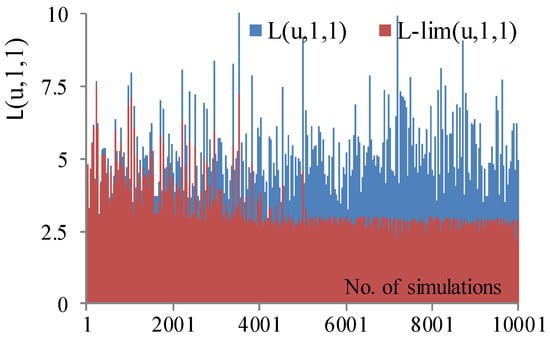
$L - l i m (u, a, b) = \{\begin{array}{l} (1 - \frac{k - 1}{k_{m a x}}) \cdot L (u, a, b), L (u, a, b) > L_{M a x} \\ L (u, a, b), otherwise \end{array}$

(15)

Figure 1 shows the first 10,000 values simulated using the Laplace operators L(u,a,b) and L-lim(u,1,1) considering the Laplace distribution parameters a = 1 and b = 1. The operator L(u,1,1), represented in blue, exhibits high values throughout the range of simulations, which could lead to excessively large search steps toward the end of the search process. In contrast, L-lim(u,1,1), represented in red, initially shows higher values (allowing for predominantly extensive exploration to identify favorable regions). However, as the number of simulations increases, the values are attenuated and plateau at the predefined maximum limit L_Max. Thus, the attenuated values of L-lim(u,1,1) favor the exploitation phase, enabling intensive searching around the current solutions.

Modifications made to the proposed SGO-L algorithm compared to SGO are as follows:

(i). In the improving phase, Equation (10) is replaced with Equation (16) in the followig form:

X_i,new = c·X_i + L-lim(u,a,b)∙r₂·(X_Best − X_i), i = 1, 2, …, N

(16)

(ii). In the acquiring phase, Equation (11) is replaced with Equation (17) in the following form:

If f(X_i) < f(X_r) Then, X_i,new = X_i + L-lim(u,a,b)∙r₃ (X_i − X_r) + L-lim(u,a,b)∙r₄ (X_Best − X_i)

(17a)

Else X_i,new = X_i + L-lim(u,a,b)∙r₃ (X_r − X_i) + L-lim(u,a,b)∙r₄ (X_Best − X_i), i = 1, 2, …, N

(17b)

(iii). The verification and update of the best solution (X_Best) will be performed after generating each solution (X_i_,new) in both the improving phase and the acquiring phase. Additionally, the value of the factor c will be considered as c = 1.

The specific improvements of the SGO-L algorithm compared to SGO result from the modifications included in the structure of SGO-L, as presented in points (i)–(iii) mentioned above. The main improvement comes from the inclusion of the Laplace operator with bounded values, L-lim(u,a,b), in the structure of the update relationships of the solutions, both in the improving phase and in the acquiring phase. This operator was introduced to generate suitable search steps during the exploration and exploitation phases of the solution space to maintain a good exploration–exploitation balance, which ultimately allows for the attainment of high-quality solutions and good stability with rapid convergence. Additionally, according to modification (iii), the update–evaluation cycle of the solutions is carried out dynamically, thus allowing for the immediate exploitation of an improved solution, resulting in an increase in the rate of convergence.

Considering the modifications (i)–(iii), the steps for applying the proposed SGO-L algorithm are presented below (Algorithm 2).

Algorithm 2: SGO-L algorithm.

Set the general parameters (N, k_max) and specific parameters (a, b, and L_Max) for SGO-L
Initialization phase
Initialize the population X_i, i = 1, 2 …, N in the social group using Equation (9)
Calculate the fitness f(X_i), then find X_Best and f(X_Best)
while k ≤ k_max
for i = 1 to N do Improving phase
Generate a value using the Laplace operator L-lim(u,a,b) using (15)
Calculate the new solution X_i_,new using Equation (16)
Calculate the fitness f(X_i_,new)
Update the solutions X_i and X_Best and their corresponding fitness values f(X_i) and f(X_Best) using greedy selection
end for
for i = 1 to N do Acquiring phase
Randomly select a solution X_r, i ≠ r
Generate a value using the Laplace operator L-lim(u,a,b) based on Equation (15)
Calculate the new solution X_i_,new using Equation (17)
Calculate the fitness f(X_i_,new)
Update the solutions X_i and X_Best and their corresponding fitness values f(X_i) and f(X_Best) using greedy selection
end for
k = k + 1
end while
Return X_Best, and the fitness f(X_Best).

The main steps of the suggested SGO-L algorithm are summarized in Figure 2 as a flowchart. Also, the modifications made to the proposed SGO-L are highlighted.

5. Implementing the SGO-L for the ED Problem

To implement the SGO-L or SGO algorithm, we consider that any solution i is represented by the power vector [P_i] = [P₁_,i, P₂_,i, …, P_j_,i, …P_m_,i] and the vector of the fuel types used [TF_i], i = 1, 2, …, N (if there are units with multiple fuel sources).

To solve the ED problem using the proposed SGO-L algorithm, Algorithm 2 (presented in Section 4) is applied, with the following additions related to handling inequality and equality constraints—relations (3)–(6) presented in the optimization model [5,12]:

(i). If the power of a unit j (P_j, j = 1, 2, …, m) is outside the operating limits (P_j_,min, P_j_,max) defined by relation (3), it is set to the exceeded limit (P_j = P_j_,min or P_j = P_j_,max);

(ii). If the power of a unit j (P_j, j = 1,2, …, m) is outside the operating limits (Max(P_j_,min, P⁰_j − DR_j), Min(P_j_,max, P⁰_j + UR_j)) defined by the combination of relations (3)–(4), it is set to the exceeded limit (P_j = Max(P_j_,min, P⁰_j − DR_j) or P_j = Min(P_j_,max, P⁰_j + UR_j));

(iii). If the power of a unit j (P_j, j = 1, 2, …, m) is within a prohibited operating zone (P^l_j_,z, P^u_j_,z) defined by relation (5), it is set to the upper limit of zone z (P_j = P^u_j_,z);

(iv). To handle the equality constraint (6), we use the solution adjustment procedure described in [5].

It should be noted that the corrections specified in points (i)–(iii) are applied to adjust each component P_j_,i of the power vector [P_i] in all phases of SGO-L (initialization, improving, acquiring). The correction from point (iv) is applied to each vector generated through Equations (9), (16), and (17), resulting in a new power vector that satisfies relation (6) with the predefined accuracy ε. The corrections specified in points (i)–(iv) are used similarly when applying the SGO algorithm to solve the ED problem. The type of fuel used, represented by the vector [FT_i], is determined based on the power intervals (known values from the problem’s input data) within which the components P_j_,i of the power vector [P_i] are placed after applying the corrections (i)–(iv).

6. Case Studies

In this section, the performance of the SGO-L algorithm is tested on four power systems with various practical characteristics, such as the valve-point effect, transmission line losses, sources with multiple fuel options, prohibited zones of generating units, and the operating limits of the generators. Based on the size and characteristics of the power systems, we study four cases mentioned in Table 1 and described below.

Case 1 (C₁): Case C₁ represents an IEEE power system with six thermal units, considering POZs, ramp rate limits, and transmission losses. The power demand is 1263 MW. The cost coefficients (a_j, b_j, c_j, j = 1, 2, …, 6) and B-loss coefficients are taken from [12] with the mention that the B₀₀ term in the loss expression has been corrected according to the details in [51].

Case 2 (C₂): This case studies a 10-unit system that considers transmission line losses and the valve-point effect. The power demand is 2000 MW. The cost coefficients (a_j, b_j, c_j, e_j, f_j, j = 1, 2, …, 10) and loss coefficients (B_ij) are taken from [52].

Case 3 (C₃): The third case analyzes a 10-unit system that considers multi-fuel sources and the valve-point effects. The power demand is 2700 MW. Input data for the generating units are taken from [14].

Case 4 (C₄): Case C4 is a large-scale system with 40 units, which considers the valve-point effects. The power demand is 10,500 MW, and the cost coefficients are taken from [50].

Case 5 (C5): The last case is a system with 110 units, which does not consider valve-point effects or transmission line losses. The power demand is 15,000 MW, and the input system data are available in [22]. For each case (C₁–C₄), 50 independent runs of the SGO and SGO-L algorithms were performed, and a set of statistical indicators was determined as follows: the best cost obtained for the objective function F (MinCost), the average cost (MeanCost), the maximum cost (MaxCost), and the standard deviation (SD). Additionally, the average execution time (Time) is presented for both the SGO and SGO-L algorithms. The accuracy of the calculations was set to ε = 10⁻⁵ MW.

Both algorithms (SGO and SGO-L) were implemented in MathCAD and executed on a computer with the following specifications: Intel i5 processor, 2.2 GHz CPU, and 4 GB of RAM.

6.1. Setting the Parameters

The tuning of metaheuristic algorithm parameters is crucial, as it significantly influences their performance. Therefore, the general parameters (k_max and N) and specific parameters (a, b, and L_Max for SGO-L) were set by conducting experimental trials. The adjustment of the parameters for the SGO and SGO-L algorithms was carried out based on the following rule: when one parameter is varied, the other parameters are kept constant. The best combination of parameter values was chosen based on the “mean cost” criterion (MeanCost item) for the objective function F[P] defined in Equation (1). The selected values for the general parameters (N, and k_max) and specific parameters (a, b, and L_Max in the case of SGO-L) are presented in Table 1.

For a fair comparison between the original SGO and SGO-L algorithms, as shown in Table 1, the values of the general parameters (k_max and N) and the number of evaluations (NE = 2N∙k_max) were chosen to be equal for each case considered (C₁–C₄). Furthermore, it was ensured that both algorithms started from the same initial points (solutions).

6.2. Results for Case C₁ (Six Units)

The best solutions for SGO and SGO-L: Table 2 shows the best solutions obtained by the original SGO and SGO-L algorithms, as well as by several competitor algorithms (MSSA [53], DHS [1], PSO [12], CBA [17], GA [12], and FA [19]). Additionally, the values of the statistical metrics (MinCost, MeanCost, MaxCost, and SD), the transmission losses (P_L), total generated power (P_G), the power demand (P_D), accuracy (ε), average execution time (Time), and the number of evaluations (NE) for the objective function defined by relation (1) are indicated. Observing the best solutions identified by SGO and SGO-L, it can be noted that they are nearly identical, with the generating units operating close to their maximum power limit (P_max). For both algorithms (SGO and SGO-L), the best operating cost of the system (corresponding to the best solution) is approximately 15,449.89952 USD/h, a slightly better value than that obtained by other algorithms listed in Table 2, such as the MSSA [53], DHS [1], and PSO [12], among others. It is worth mentioning that the best solutions obtained by SGO-L have very high accuracy, with Accuracy < 1.0 × 10⁻⁸ MW.

Quality and stability of solutions: The solutions obtained by SGO and SGO-L are evaluated through the statistical metrics (MinCost, MeanCost, MaxCost, and SD) presented in Table 2. Examining these values reveals that the proposed SGO-L algorithm identifies higher-quality solutions than the competitor algorithms mentioned in Table 2 (SGO, MSSA [53], DHS [1], PSO [12], CBA [17], GA [12], and FA [19]). Additionally, the stability of SGO-L is excellent (with SD = 7.56 × 10⁻⁵ USD/h) considering that a relatively large number of independent runs—50 in total—were performed. Compared to the competitor algorithms listed in Table 2, SGO-L exhibits superior stability. Furthermore, the maximum value obtained by SGO-L (MaxCost = 15,449.899525 USD/h) is better than the average value (MeanCost) identified by the competitor algorithms in Table 2.

Computation time: For both algorithms (SGO and SGO-L), the computation time (Time) is very good, being approximately 0.07 s per run, which is better than the times achieved by the competitor algorithms. The only exception is the DHS [1] algorithm, which achieves a slightly lower execution time compared to SGO and SGO-L.

6.3. Results for Case C₂ (10 Units)

The best solutions for SGO and SGO-L: Table 3 presents the best generation scheduling solutions obtained by the SGO and SGO-L algorithms, as well as several competitor algorithms (IPOA [24], OMF [54], PSO [22], HHO [22], ISMA [22], and CSCA [21]).

From the solutions obtained by the algorithms listed in Table 3, it is observed that most generators (P₁, P₂, P₇–P₁₀) operate at maximum capacity, with differences between the solutions identified by the mentioned algorithms being attributable to units P₃–P₆. The best operating cost is achieved by the proposed SGO-L algorithm (MinCost = 111,497.63013 USD/h), but very similar values are also identified by other algorithms, such as SGO, OMF [54], PSO [22], the ISMA [22], or the CSCA [21]. An exception is observed for the IPOA [24] and HHO [22] algorithms, which result in higher operating costs.

Quality and stability of solutions: From Table 3, it can be seen that the proposed SGO-L algorithm outperforms all competitor algorithms, achieving a better set of quality values for cost indicators (MinCost, MeanCost, MaxCost, and SD). The very low values of the SD indicator (SD_SGO-L = 7.56 × 10⁻⁵ USD/h) indicate excellent stability for the SGO-L algorithm.

Since the SD values obtained by SGO-L are lower than those achieved by competitor algorithms, SGO-L demonstrates superior stability. Similarly to Case C₁, the maximum value obtained by SGO-L (MaxCost = 111,497.63049 USD/h) is better than the mean cost, MeanCost (and very close to the minimum cost, MinCost), identified by the competitor algorithms in Table 3.

Computation time: For both algorithms (SGO and SGO-L), the average execution time (Time) is excellent, being approximately 0.09 s per run, which is better or significantly better than the time achieved by the competitor algorithms. This can also be observed from the fact that SGO-L requires a small number of evaluations (NE = 1400) of the objective function to reach the optimal solution compared to the competitor algorithms in Table 3, which require a much higher number of evaluations, NE > 15,000).

6.4. Results for Case C₃ (10 Units with Multi-Fuel)

The best solutions for SGO and SGO-L: The best results obtained by SGO and SGO-L for the scheduling of generating units with multiple fuel sources are presented in Table 4. For this case, the solution consists of the unit power outputs (P₁–P₁₀) and the type of fuel used. Both SGO and SGO-L identify the same fuel types for the obtained solutions. The accuracy of the power balance—relation (8)—corresponding to the solutions identified by SGO and SGO-L is high, with accuracy < 2 × 10⁻⁶ MW. The best operating cost is achieved by SGO-L (MinCost = 623.82940 USD/h), which is better than the cost identified by SGO or other algorithms mentioned in Table 5.

Quality and stability of solutions: From Table 5, it can be observed that the statistical indicators (MinCost, MeanCost, MaxCost) obtained by SGO-L have lower values than those obtained by SGO or other competitor algorithms listed in the table. Thus, SGO-L outperforms both well-known algorithms (such as PSO [13], DE [15], CSA [16], BSA [18], or FA [19]) and algorithms obtained through various hybridization techniques (such as Jaya-SML [20], IJaya [55], GHS [56], IFA [58], MCSA [59], etc.) in terms of cost. Additionally, the stability of SGO-L is excellent (SD = 0.043 USD/h), as determined from 50 independent runs. Compared to the competitor algorithms listed in Table 5, SGO-L exhibits better stability than most (CSA [16], GC-Jaya [55], FA [19], etc.). However, a few algorithms (PSO [13], DE [15], Jaya-SML [20], and IJaya [55]) demonstrate better stability than SGO-L, but their solution quality in terms of cost is lower.

Computation time: The average computation time achieved by SGO and SGO-L is excellent (approximately 0.6 s/rulare), which is lower than the majority of computation times obtained by competitor algorithms. Exceptions include the BSA [18] and M_DE [57] algorithms, which have slightly better computation times but worse cost indicators (MinCost, MeanCost, and MaxCost).

6.5. Results for Case C₄ (40 Unit)

The best generation scheduling results identified by the SGO and SGO-L algorithms are presented in Table 6. In cases C1-C3, which analyze small- and medium-sized systems, the best solutions obtained by SGO and SGO-L are very close (cases C₁ and C₂) or similar (case C₃); in case C₄ (which studies a large-scale system with 40 units with VPE), the solutions and operating costs identified by the two algorithms differ significantly (MinCost_SGO = 121,492.1621 USD/h and MinCost_SGO-L = 121,420.9436 USD/h). The accuracy of satisfying the power balance is very high for both algorithms, with Accuracy < 2 × 10⁻¹¹ MW. Additionally, the best solution obtained by SGO-L is better than the solutions identified by SGO or other competitor algorithms listed in Table 7 (except the ESNS algorithm [3], which achieves a slightly lower minimum cost).

Quality and stability of solutions: Table 7 presents the statistical cost indicators (MinCost, MeanCost, MaxCost, and SD) obtained by SGO, SGO-L, and other competitor algorithms. The proposed SGO-L algorithm outperforms all competitor algorithms listed in Table 7 in terms of cost indicators. The stability of SGO-L is good (SD_SGO-L = 75.89 USD/h) compared to the stability achieved by other algorithms, where (SD ranges between 160.88 USD/h and 866.20 USD/h). Additionally, the number of evaluations NE performed by SGO-L is relatively small compared to the NE required by other algorithms, where NE > 40,000 (with the exceptions of SMA [61] and SCA [62]).

Computation time: The average computation time (item Time) achieved by SGO and SGO-L is excellent (approximately 4 s per run), being better than the algorithms listed in Table 7.

6.6. Results for Case C₅ (110 Unit)

The best solutions for SGO and SGO-L: The best solutions obtained using the SGO and SGO-L algorithms are shown in Table 8. The minimum cost achieved by SGO-L (MinCost_SGO-L = 197,988.1782 USD/h) is more competitive than that identified by SGO (MinCost_SGO = 197,990.3133 USD/h). The accuracy of satisfying the power balance for the best solutions identified by both SGO and SGO-L is very high, with accuracy < 2 × 10⁻¹¹ MW. Additionally, the best solution obtained by SGO-L is better than the solutions identified by SGO or other competitor algorithms listed in Table 9.

Quality and stability of solutions: From Table 9, the performance of the proposed SGO-L algorithm (for the 110-unit system) can be observed in comparison to SGO and other competing algorithms in terms of cost (MinCost, MeanCost, MaxCost, and SD) and execution time (item Time).

The proposed SGO-L algorithm outperforms all competitor algorithms listed in Table 9 in terms of cost and execution time (except for the TFWO algorithm [36], which achieves slightly better values for MeanCost and MaxCost. Notably, SGO-L demonstrates superior capabilities in extracting high-quality and highly stable solutions compared to well-known algorithms (such as PSO [31], CSO [31], SMA [22], HHO [22], SNS [3], GWO [3], and SOS [35]) and improved versions of these algorithms (e.g., OLCSO [31], ISMA [22], ESNS [3], DSOS [35]).

The stability of SGO-L is very good (SD_SGO-L = 0.0048 USD/h) compared to the stability achieved by the majority of algorithms in Table 9, for which the SD ranges between 144.44 USD/h and 3248.17 USD/h. A few algorithms exhibit good stability (SD < 1 USD/h), but their cost indicators are higher than those of SGO-L (with the exception of TFWO [36]). Additionally, the number of evaluations (NE) performed by SGO and SGO-L is significantly smaller (NE_SGO-L = 21,000) compared to the NE (>320,000) required by other algorithms.

Computation time: The average computation time (item Time) achieved by SGO and SGO-L is excellent (approximately 5 s per run), being significantly better than the algorithms listed in Table 9. The results highlighted in this paragraph emphasize the potential of the SGO-L algorithm for solving the ED problem in large-scale systems.

6.7. Comparison of SGO-L with SGO and Other Algorithms

SGO versus SGO-L: In all studied cases (C₁–C₅), the statistical cost indicators (MinCost, MeanCost, MaxCost, and SD) obtained by SGO-L are superior to those obtained by SGO (see Table 2, Table 3, Table 5, Table 7 and Table 9 corresponding to cases C₁, C₂, C₃, C₄, and C₅). However, to demonstrate the positive influence of including the Laplace distribution in the solution update equations of SGO-L and to show that SGO-L achieves statistically significantly better results than SGO, a comparison of the two algorithms is performed using the non-parametric Wilcoxon statistical test. The Wilcoxon test is applied with a significance level of 1%, and the number of value pairs being compared is equal to 50. Practically, each algorithm (SGO or SGO-L) performs 50 runs for each case study. The Wilcoxon test is applied for two related samples using the SPSS^® software package, version 16 (Statistical Package for the Social Sciences).

Table 10 presents the p-value items resulting from the application of the Wilcoxon test for comparing the value pairs corresponding to the SGO and SGO-L algorithms. In all cases, the p-value is below 0.01, indicating that the costs obtained by SGO-L are significantly better than those obtained by SGO. The test results demonstrate that including the Laplace distribution in SGO-L has positive effects, leading to increased performance of this algorithm compared to SGO.

Convergence process: The convergence characteristics of the SGO and SGO-L algorithms, as a function of the number of iterations, are shown in Figure 3a–e corresponding to the five studied cases. In all studied cases (C₁–C₅), the convergence of both SGO and SGO-L is rapid. The objective function decreases sharply during the first (15–20)% of the maximum number of iterations, followed by a very slow decrease, and the iterative process stabilizes. From Figure 3a–e, it can be observed that SGO converges slightly faster than SGO-L during the initial iterations (in C₁–C₄ cases) because SGO has good global search capabilities. However, as the iterative process progresses, SGO-L, equipped with the Laplace distribution, performs better local searches than SGO and ultimately identifies better solutions. The best solutions identified by SGO and SGO-L (MinCost) are presented in Table 2, Table 3, Table 5, Table 7 and Table 9. It should be noted that the plotted characteristics correspond to the best solutions found in each studied case.

To more clearly highlight the superior local search capability of the proposed SGO-L algorithm compared to SGO and the transition from the exploration phase to the exploitation phase, we present the variation in the objective function with the number of evaluations (NE) performed (Figure 4a–f) for each case. From Figure 4a–f—the area marked in blue—it can be observed that SGO maintains a high global search capability throughout the iterative process, with the values of the objective function remaining high both in the initial and final iterations. Thus, SGO is unable to focus during each run on a potential area that could later be exploited intensively to extract a near-optimal or optimal solution.

However, it should be noted that SGO does perform an exploitation phase, albeit in a more limited form (in all cases, several solutions are generated around the current best solution—see, for example, Figure 4f, where the lower blue area indicates this observation). Additionally, Figure 4f reveals a large blue area/band that highlights the multitude of high costs generated by solutions potentially that are far from the current best solution. This large blue area in Figure 4f demonstrates that a significant portion of the solutions generated by SGO result in high costs and inefficiencies due to the fact that they provide information with low potential for identifying profitable areas. These blue zones/bands, characteristic of the SGO algorithm, appear in all the studied cases, indicating that SGO does not perform sufficiently intensive local searches. Thus, in case C₁—Figure 4a—three blue areas appear; in C₂—Figure 4b—four distinct blue areas are visible; in C₃—Figure 4c—four distinct areas are observed; in C₄—Figure 4d—five distinct areas are present; and in C₅—Figure 4e—two distinct areas are identified (in each case, the lower blue area—associated with low-cost values—is partially obstructed by the red area corresponding to the costs obtained by the SGO-L algorithm).

In contrast, observing the behavior of SGO-L (the area marked in red in Figure 4a–e), it can be seen that it initially executes successful global searches (exploration phase) and then transitions to an intense local search (exploitation phase) around the current solutions. Thus, for all the studied cases, the SGO-L algorithm can achieve solutions that are very close to or near the optimal solution. From Figure 4a–e (the areas corresponding to the points marked in red), it can be observed that in all cases, the cost values of the solutions generated by SGO-L remain close to the best current solution. As a result, the SGO-L algorithm is characterized by a unique, stable, and narrow or relatively narrow red zone (for case C₄) with a continuous decrease. These features indicate that SGO-L performs an intensive local search throughout the entire iterative process. Practically, SGO-L manages to capture a greater amount of useful information than SGO by translating solutions from the blue zone into the red zone, where the corresponding costs are lower. This is due to the inclusion of values generated by the Laplace distribution in the structure of the solution update equations (values that are limited to a maximum threshold, L_Max).

When the parameters of the Laplace distribution are properly tuned, this distribution can generate suitable steps both in the global search phase and in the local search phase, leading to high-quality and stable solutions for small-, medium-, and large-sized ED problems (including convex functions in the case of the 110-unit system). For large-scale ED problems (such as case C₄, 40-unit system), the use of the Laplace distribution in SGO-L results in acceptable solutions. Given the results obtained, the Laplace distribution could be successfully incorporated to enhance the characteristics of other classical or recently proposed metaheuristic algorithms.

Cost saving is calculated based on the mean cost, in USD/year, using the following equation: CostSaving = (MeanCost_C − MeanCost_SGO-L)8760, where MeanCost_C is the mean cost obtained from 50 runs of a given competitor algorithm C and MeanCost_SGO-L is the mean cost obtained from 50 runs of SGO-L. Table 2, Table 3, Table 5, Table 7 and Table 9 present the Cost Saving values corresponding to cases C₁, C₂, C₃, C₄, and C₅, respectively. For small-scale systems (case C₁, six-unit system) and medium-scale systems (C₂ and C₃, 10-unit systems), the cost saving is minor (as most competitor algorithms are capable of obtaining solutions relatively close to the optimal solution), with a few exceptions, such as the CBA [17] (in case of C₁), HHO [22] (case C₂), or IGA-MU [14] (in case of C₃). However, in the case of C₄ or C₅, which is a large-scale system, the cost saving is more significant.

Discussion on computation time: The comparison between SGO-L and competitor algorithms in terms of the time metric should be regarded as indicative, as the algorithms were executed on different computing systems or, in some cases, due to the lack of information about these systems. Nevertheless, in most cases, the difference in execution times achieved by SGO-L compared to the competitor algorithms is evident. Additionally, SGO-L requires a significantly smaller number of evaluations (NE) compared to the competitor algorithms (e.g., PSO [12], GA [12], FA [19] in case C1; PSO [22], HHO [22], ISMA [22] in case C2; SOA [60], EBWO [60], ESCSDO [23] in case C4; and all algorithms in case C5). Consequently, the execution time of SGO-L should be shorter than that of the mentioned competitor algorithms provided that the computing systems used have similar characteristics.

7. Conclusions

This article introduces a new variant of the SGO algorithm, denoted as SGO-L, achieved by integrating the Laplace operator into the heuristics implemented in the improving and acquiring phases. The aim is to regulate the search steps in the solution space and enhance the exploration–exploitation balance, positively impacting the quality and stability of the solutions obtained through SGO-L. SGO-L was successfully validated on four systems of small (six units), medium (10 units), and large (40 units) sizes. In all analyzed cases (C₁–C₄), statistical tests show that SGO-L outperforms the SGO algorithm, achieving higher quality and more stable solutions.

In cases corresponding to small (C₁, six units) and medium (C₂, 10 units) systems, SGO and SGO-L achieve very close values for the MinCost indicator, but SGO-L is superior for other indicators (MeanCost, MaxCost, and SD). SGO-L’s superiority becomes more evident in larger cases (C₄, 40-unit systems), where the entire set of statistical indicators (MinCost, MeanCost, MaxCost, and SD) shows significant improvements over SGO. Moreover, the annual cost savings exceed USD 4 million in the case of C4.

Both algorithms, SGO and SGO-L, achieve excellent average execution times; for instance, in the 40-unit system, the Time indicator is below 4.1 s per run compared to other algorithms exceeding 19 s per run. SGO-L demonstrates better average performance and stability than well-known algorithms (e.g., PSO, FA, DE) and modern competitors (e.g., SNS, TLABC, EBWO).

The results confirmed through statistical tests show that equipping SGO-L with the Laplace operator brings significant improvements compared to SGO in solving the ED problem. The main disadvantage of the Laplace operator lies in the need to tune its specific parameters (a, b, and L_Max), which can significantly impact the quality of the solutions.

The SGO-L algorithm is characterized by its simplicity, ease of understanding and implementation, rapid convergence, and flexibility for hybridization with other algorithms. Additionally, SGO-L has the ability to identify high-quality and stable solutions for small- and medium-sized systems with non-convex functions and for large-scale systems with convex functions (110 units). However, for large-scale systems with non-convex functions, the performance of SGO-L is moderate in terms of stability, indicating the need for further improvements to the algorithm.

Future work could explore the potential of the Laplace operator within SGO in other forms (as a mutation and/or crossover operator) or in combination with other metaheuristic algorithms. We will also test whether the Laplace operator maintains its efficiency when incorporated into the structure of other metaheuristic algorithms. The new versions obtained can be applied without limitation, for example, in power system optimization (such as multi-area ED, dynamic ED, ED problems with renewable sources, hydrothermal scheduling, etc.), in other fields, or for optimizing complex mathematical functions.

Source link

Dinu Calin Secui www.mdpi.com

Greenberg News

A Social Group Optimization Algorithm Using the Laplace Operator for the Economic Dispatch Problem

1. Introduction

2. Statement of the ED Problem

3. Social Group Optimization (SGO)

4. Modified SGO Operator Laplace (SGO-L)

5. Implementing the SGO-L for the ED Problem

6. Case Studies

6.1. Setting the Parameters

6.2. Results for Case C₁ (Six Units)

6.3. Results for Case C₂ (10 Units)

6.4. Results for Case C₃ (10 Units with Multi-Fuel)

6.5. Results for Case C₄ (40 Unit)

6.6. Results for Case C₅ (110 Unit)

6.7. Comparison of SGO-L with SGO and Other Algorithms

7. Conclusions

Greenberg

1. Introduction

2. Statement of the ED Problem

3. Social Group Optimization (SGO)

4. Modified SGO Operator Laplace (SGO-L)

5. Implementing the SGO-L for the ED Problem

6. Case Studies

6.1. Setting the Parameters

6.2. Results for Case C1 (Six Units)

6.3. Results for Case C2 (10 Units)

6.4. Results for Case C3 (10 Units with Multi-Fuel)

6.5. Results for Case C4 (40 Unit)

6.6. Results for Case C5 (110 Unit)

6.7. Comparison of SGO-L with SGO and Other Algorithms

7. Conclusions

Related Posts

An Alternative to the Bland—Altman Repeated-Measures Correlation to Account for Variability of Slopes Across Persons

Environmental Factor – March 2021: Chronic lung disease responds to hyaluronan in NIEHS-led study

Editorial on the Special Issue Titled “Pathology and Diagnosis of Gynecologic Diseases—2nd Edition”

Greenberg

6.2. Results for Case C₁ (Six Units)

6.3. Results for Case C₂ (10 Units)

6.4. Results for Case C₃ (10 Units with Multi-Fuel)

6.5. Results for Case C₄ (40 Unit)

6.6. Results for Case C₅ (110 Unit)