
1. Introduction
When a data set includes repeated measures, i.e., multiple measurements taken for each person, estimating a correlation between two variables requires separation of variance within and across persons. This is necessary because standard Pearson correlations assume that each observation is independent of all others, but this assumption is violated when multiple measurements come from the same person. When we have repeated measurements from individuals, observations within each person are naturally more similar to each other than to observations from different people. This creates a hierarchical or nested data structure where measurements are clustered within individuals. If we simply calculated a Pearson correlation across all data points while ignoring this nesting, we would conflate two distinct sources of variation: the differences between people’s average levels (between-person variation) and the relationships between variables within each person over time (within-person variation). For example, imagine we are studying the relationship between exercise and mood. Some people might generally exercise more and have better moods overall, creating a positive between-person correlation. However, the relationship we are often really interested in is whether an individual person’s mood improves when they exercise more than their personal average—the within-person correlation. By using a repeated-measures correlation, we can specifically examine these within-person relationships while accounting for the fact that each person has their own baseline levels and patterns. This gives us a more accurate understanding of how variables relate to each other at the individual level, rather than mixing this information with broader patterns that exist across different people.
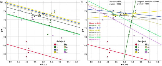
Here, we propose an alternative to the Bland–Altman rmcorr. Specifically, we propose calculating all within-person correlations, taking the average of them weighted by the square root of the within-person observations, and testing this weighted average for statistical significance using a one-sample t-test also weighted by the square root of the observations. We recommend that researchers use both this method and the original Bland–Altman method for comparison. As we demonstrate below, an extreme inconsistency between these two estimates could suggest methodological or data quality problems that should be addressed before further statistical analyses are conducted.
4. Discussion
We propose an alternative to the Bland–Altman repeated-measures correlation (rmcorr) for estimating within-person correlations between two variables in a repeated-measures data set. Our proposed method, the weighted mean within-person correlation (wmcorr), calculates the average of all within-person correlations, weighted by the square root of the number of observations for each person. We demonstrate that in most cases, rmcorr and wmcorr will yield similar results; however, in cases where subjects have at least moderately varying slopes, wmcorr may provide a more visually intuitive estimate of the within-person correlation. Further, simulation results showed that while wmcorr had less statistical power than rmcorr (reducing Type I errors), neither method exhibited systematic bias in estimating correlations; however, wmcorr demonstrated superior accuracy, particularly when sample sizes or true correlations were low, as evidenced by its smaller error variability (SD = 0.086 vs. 0.108). While we call wmcorr an “alternative” because it could be used as a standalone method, we encourage researchers to estimate both wmcorr and the original rmcorr. Conflicting significance levels or opposite directions of rmcorr and wmcorr can serve as “warning signs” for researchers, indicating potential data quality issues or the need for further data collection before drawing conclusions about within-person relationships.
The method proposed here shares some fundamental characteristics with mixed-effects regression models, but differs in important technical aspects. Both methods aim to account for the nested structure of repeated-measures data and focus on within-person relationships, although mixed-effects models also provide between-subject effects. The weighting by square root of sample size in the proposed approach parallels how mixed models naturally give more weight to subjects with more observations, as these subjects provide more reliable information about within-person patterns. However, the methods diverge in their underlying “machinery” and assumptions. Mixed-effects regression explicitly models both fixed and random effects, allowing for variation in both intercepts and slopes across individuals, while simultaneously estimating an overall population-level relationship. It achieves this through sophisticated maximum likelihood estimation that considers the entire data structure. Our method, by contrast, takes a two-stage approach, first calculating individual correlations, and then combining them through weighted averaging. This makes our method more computationally straightforward and potentially more intuitive to researchers, because it is clear how each person’s data contributes to the final estimate. It also avoids some of the complex assumptions about the distributions of random effects that mixed models require. However, this simplicity means our method might be less efficient at using all available information in the data, particularly when some subjects have very few observations or when there are missing data patterns that mixed models could handle more elegantly through their likelihood-based framework.
Source link
Tyler M. Moore www.mdpi.com