1. Introduction
Vehicle emissions represent a global environmental challenge, as they directly contribute to local air pollution and global warming [
1]. This impact results from the release of various components during the combustion process, which depend directly on the type of vehicle and fuel used [
2]. For instance, diesel vehicles tend to emit higher amounts of nitrogen oxides (NOx) and particulate matter (PM) [
3], while gasoline vehicles release more carbon dioxide (CO
2) and hydrocarbons (HCs) [
3,
4].
These components have adverse effects on human health, causing premature deaths and impacting domestic fauna, vegetation, and water resources in urban areas [
5,
6,
7]. In Ecuador, vehicle emissions have also been studied and characterized, reporting the magnitude and spatial distribution of these pollutants. In 2021, the country generated approximately 33 million tons of CO
2, with vehicular emissions being the second-largest contributing factor [
8]. Although this study focuses on CO
2 and hydrocarbon (HC) emissions, it is important to consider other pollutants, such as carbon monoxide (CO) and NOx, due to their environmental impact. For example, a 2019 Ecuadorian inventory recorded 109.09 T/y of CO and 13.66 T/y of non-methane hydrocarbons (NMHCs), with four-stroke motorcycles contributing 30% of CO and 24% of NMHCs [
9]. Likewise, the city of Guayaquil estimated annual emissions of 237.1 KT of CO, 46.4 KT of NOx, and 28.5 KT of volatile organic compounds (VOCs), with gasoline-powered light vehicles accounting for over 85% of CO and VOC emissions [
10].
Although the effects of vehicular emissions remain concerning, significant advancements have been made in this field over the past six decades, leading to a substantial reduction in the release of pollutants into the environment, particularly NOx, PM, CO
2, and lead, despite the noticeable increase in vehicle circulation and mileage [
6,
11]. Consequently, air quality measures have improved in countries like the United States and Europe to comply with increasingly stringent regulatory standards [
12]. However, despite these advancements, challenges persist in specific contexts. For instance, studies indicate that vehicular gas emissions are higher in densely populated areas, maritime ports, and state highways during peak hours [
8].
In this context, altitude emerges as a key factor in the study of vehicular emission variations. In Andean cities located above 2000 m above sea level (m.a.s.l.), lower atmospheric pressure, combined with the growth of the vehicle fleet, could intensify CO
2 and hydrocarbon concentrations [
8,
13,
14]. These assumptions suggest that for global advancements in emission reduction to be effective, it is necessary to explore how these specific geographical conditions influence this phenomenon. This will allow for the optimization of control strategies in high-altitude areas and will contribute to the sustainability and technological development of the automotive sector in less-studied environments [
13,
15].
Data exploration faces challenges when addressing the diversity and insufficiency of information, as conventional statistical methods fail to simultaneously capture the influence of multiple factors (e.g., manufacturing year, brand, and operating conditions) [
16]. These limitations, combined with the uncertainty generated by the volume and speed of non-representative data, hinder the design of effective policies and increase the risk of erroneous conclusions [
16,
17]. To address these issues, methods have been developed to extract multidimensional patterns and describe common properties in complex datasets, thereby justifying the application of robust statistical methods [
17,
18]. In this context, multivariate exploration approaches, such as STATIS, enable the analysis of multiple sets of variables measured on the same observations, even if they vary in quantity or nature. Although the sample size may be small or the data heterogeneous, STATIS integrates these datasets into an optimal weighted average and, through dimensionality reduction, reveals the common structure among observations, provided that the starting factor (k-tables) is well represented [
19].
This study aims to perform a statistical exploration of vehicle emissions from gasoline-powered cars in Guaranda (Ecuador) as an initial step to identify underlying patterns by using the tripartite STATIS method. A three-way table has been constructed, integrating (i) vehicle model year intervals (across six tables), (ii) vehicle brand and model, and (iii) four gas emission indicators. This work focuses exclusively on CO2 (CD) and hydrocarbon (HC) emissions measured under idle (ICD and IHC) and dynamic conditions (HCD and HHC), excluding analyses of particulate matter or other factors such as tire wear. This approach seeks to provide insights into the influence of these factors on emissions, particularly in a high-altitude environment like Guaranda, and to lay the groundwork for designing more targeted and effective emission control strategies.
2. Materials and Methods
In this study, a sample of 79 gasoline-powered vehicles was examined to evaluate carbon dioxide (CO2) and hydrocarbon (HC) emissions under idle and dynamic conditions, aiming to explore the effects of factors such as model, brand, and model year. For the objectives and analyses, the data obtained were labeled ICD (CO2 emissions under idle conditions), IHC (HC emissions under idle conditions), DCD (CO2 emissions under dynamic conditions), and DHC (HC emissions under dynamic conditions).
2.1. Design and Sample
This study is exploratory in nature, with a cross-sectional and analytical design, seeking to analyze the relationships and effects of triple-entry factors (model–brand, year, and indicators) on vehicle gas emissions. Representative vehicles from the studied fleet were selected, ensuring their mechanical condition, particularly the integrity of their exhaust systems.
The selection criteria for this study included gasoline-powered vehicles with specified model, brand, and model year. Additionally, the vehicles evaluated were predominantly mid-range models equipped with naturally aspirated engines. This choice reflects the composition of Ecuador’s automotive fleet, where approximately 75% of vehicles are mid-range and commonly feature naturally aspirated engines, as reported by Instituto Nacional de Estadística y Censos (INEC) and Agencia Nacional de Tránsito (ANT) [
20]. Finally, it was ensured that the vehicles had been previously fueled with Extra gasoline (87 octane), the standard fuel in Ecuador for internal combustion engines. Although the refueling was not conducted by the research team, nationwide regulations guarantee consistent fuel quality and composition across all service stations, thereby minimizing any variability in emissions due to fuel differences.
Vehicles were excluded if they were diesel-powered, lacked complete technical specifications, or presented mechanical issues that could compromise emission readings. From a total of 150 vehicles evaluated at the Guaranda station, the process resulted in a sample of 79 vehicles with characteristics suitable for inclusion in a triple-entry dataset. These selection criteria ensured data consistency and the mechanical integrity necessary for accurate emission testing, though they may limit the generalizability of the findings to the broader vehicle fleet.
Prior to measurements, visual inspections and checks were conducted to rule out defects that could compromise results, as recommended by [
21]. The evaluation process followed technical standard RTE INEN 017:2008 [
22].
2.2. Procedure and Measurements
The measurement of the indicators (ICD, IHC, DCD, and DHC) was carried out by using an LPS 3000 VP186010 console (MAHA Maschinenbau Haldenwang GmbH & Co. KG, Haldenwang, Germany). This equipment features an integrated constant volume sampling (CVS) system, ensuring representative emission collection through a direct connection to the vehicle’s exhaust pipe.
2.2.1. Idle Test (ICD and IHC)
For the idle tests, a minimum idle threshold was established, chosen according to the specifications of the manufacturer or assembler. When such specifications were unavailable, a maximum of 1100 r.p.m. was defined. The vehicles were then started and maintained at idle speed without load, in neutral (for manual transmissions) or in park (for automatic transmissions). The engine temperature was monitored to ensure it reached the normal operating temperature, defined as at least 75 °C in the oil pan or after running for a minimum of 10 min. Finally, CO2 (ICD) and HC (IHC) concentrations (measured in % vol.) were recorded by using a constant volume sampling (CVS) system and calibrated gas analyzers.
2.2.2. Dynamic Test (DCD and DHC)
Dynamic emission measurements were conducted by using a dynamometer (LPS 3000, MAHA Maschinenbau Haldenwang GmbH & Co. KG, Haldenwang, Germany) and the FTP-75 cycle, a standardized dynamic driving cycle used to evaluate vehicle emissions. This cycle consists of three phases: cold-start transient (505 s), stabilized (864 s), and hot-start transient (505 s). During the latter, vehicles undergo accelerations, braking, and constant speeds [
14]. A single real-time concentration was recorded for each vehicle throughout all cycle stages (measured in ppm vol.).
2.3. Study Area
This study was conducted in the city of Guaranda, Ecuador, located at an altitude of 2668 m above sea level (m.a.s.l.), which provides unique geographical conditions that can alter vehicle gas emission behavior (23). Recent studies have highlighted the importance of investigating vehicle emissions in high-altitude regions, as CO
2 emissions increase significantly with elevation, reaching up to three times their normal levels [
15]. Both diesel and gasoline vehicles exhibit higher emission factors at greater altitudes, with atmospheric pressure being the main environmental factor affecting this phenomenon. Additionally, vehicle speed and acceleration also play significant roles [
23,
24].
The variables included in this study, such as the model and primarily the brand, were used as input factors for the STATIS analysis (see
Section 2.4), facilitating data coding and organization. While the brand does not serve as a direct explanatory factor, its influence groups consistent technical characteristics, such as engine technology and vehicle configuration. Additionally, altitude was not considered a differentiating variable, as all vehicles were evaluated under the same atmospheric condition, ensuring that atmospheric pressure affected all vehicles uniformly and minimizing its impact on engine performance.
2.4. Statistical Analysis
The objective of this study is to explore gas emission levels by using efficient multivariate methods, specifically the “principal component analysis” (PCA)-based STATIS model [
18]. This section describes the applied techniques, which are supported in the literature as effective data exploration methods. Systematic analysis was performed by using version 4.4.1 of R, incorporating descriptive results (mean and standard deviation) for explanatory data analysis.
STATIS
Exploratory data analysis reported in the literature is extensive, especially concerning unidimensional response datasets, such as CO
2 and hydrocarbon levels. STATIS is a multivariate exploratory data analysis technique grounded in linear algebra, particularly in Euclidean vector spaces. Its name is derived from the French expression “Structuration des Tableaux à Trois Indices de la Statistique”, meaning the “structuring of three-way statistical tables”, and it is also known by the acronym ACT (“Analyse Conjointe de Tableaux”) [
25].
The analysis was based on the dataset resulting from vehicle evaluations conducted at the Guaranda station during the period 2023–2024. Four types of gas measurements were considered: ICD, IHC, DCD, and DHC. The selection of these criteria was directed by the capabilities of the measurement equipment used. The vehicular data, including brand and model, exhibited substantial diversity in terms of population, making STATIS the preferred method over other tripartite approaches, such as PTA. For instance, while PTA is suitable for modeling specific variations among conditions, STATIS allows for the exploration of a global common structure across multiple tables, aligning better with the study’s objectives.
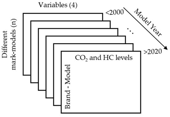
The data were organized as follows (see
Figure 1), following the recommendations of [
19,
26]:
Objects (n): Combinations of vehicle brands and models.
Variables (p): The four gas evaluation conditions (ICD, IHC, DCD, and DHC).
Temporal Dimension (k): Six intervals corresponding to the manufacturing years of the vehicle models studied.
STATIS is a method that extends principal component analysis (PCA), specifically designed to analyze multiple sets of variables collected from the same observations. This method is developed in three key stages, allowing for the decomposition and synthesis of the information contained in the data [
19,
25,
27].
In the first stage, known as
Interstructure, the relationships among the various datasets are analyzed by using similarity measures, such as the scalar product between tables. This initial analysis identifies how individual configurations relate to one another and establishes comparisons [
19]. The second stage, referred to as
Compromise, integrates the datasets into a combined representation, calculated as an optimal weighted mean of the individual configurations. This global representation, called the Compromise, is subsequently analyzed by using PCA to identify the common structure among the observations, maximizing correlation with each original configuration [
19,
28]. Finally, in the third stage, known as
Trajectories or
Intrastructure, the original datasets are projected onto the Compromise. This process enables the exploration of both similarities and discrepancies among the original configurations [
25,
27].
All mathematical operations involved in this statistical method, such as two-dimensional representations, component extraction, and the calculation of coordinates corresponding to model years, brands, and brand–model combinations, were performed by using the “ade4” package within the R environment, version 4.1 (2024) [
29].
3. Results
3.1. Descriptive Statistics
The mean values and standard deviations of gas emissions are summarized in
Table 1 and
Table 2, organized by model and manufacturing year, respectively. The descriptive analysis of carbon dioxide (CO
2) and hydrocarbon (HC) emissions across various vehicle models, under idle and high-revolution conditions, reveals varying levels of response.
Among the analyzed brands, Chevrolet represents 41.78% of the total analyzed sample, with the Aveo model having the highest frequency of use (12.7%), followed by the Corsa model. The latter showed the highest average CO2 emissions, with values of 1.42 ± 1.47% vol. under idle conditions (ICD) and 1.91 ± 1.84% vol. at high revolutions (DCD). Regarding HC emissions, the Luv model recorded the highest concentrations, reaching 322.5 ± 109.15 ppm vol. under idle conditions (IHC) and decreasing to 257 ± 121.92 ppm vol. at high revolutions (DHC).
These patterns are consistent across other models. For example, in the Toyota brand, the Stout model stands out with the highest levels in all four indicators: ICD of 2.01, DCD of 1.01, IHC of 240, and DHC of 203 (see
Table 1).
The analysis of model years (see
Table 2) reveals the average levels of CO
2 and HC emissions under idle and high-revolution conditions. Most of the vehicles evaluated in Guaranda fall within the 2010–2015 model range (34.18%), followed by the 2006–2009 range (21.52%). In contrast, models manufactured before the year 2000 represent the lowest frequency (5.06%) but exhibit the highest values across all four indicators: ICD of 3.18% vol., DCD of 3.56% vol., IHC of 414 ppm vol., and DHC of 334.75 ppm vol.
This indicates that although relatively few users operate such older vehicles, these contribute significantly to pollutant gas emissions. The analysis also reveals a decreasing trend in CO2 and HC emissions as the model years progress. For example, vehicles manufactured before 2000 record average CO2 emission levels close to 3% vol. and HC emissions around 400 ppm vol. In contrast, vehicles manufactured after 2020 show much lower levels, with averages of 0.27% vol. for CO2 and 100 ppm vol. for HC.
3.2. Interstructure Analysis
The first step of STATIS (Interstructure) examines the similarities among the six model year intervals analyzed concerning gas emission evaluations. This is based on the calculation of the RV coefficient matrix.
Table 3 presents these coefficients.
Analyzing the RV coefficients in
Table 3 reveals that the model year intervals with the highest similarities are those between 2000 and 2005 and post-2020 models, as well as models from 2016 to 2019, with RV coefficients of 0.96 and 0.941, respectively. Conversely, the least correlated models or those with the most distinct patterns are found between pre-2000 models and the most recent models, specifically those from 2010 to 2015 and 2016 to 2019, with RV coefficients of 0.53 and 0.406, respectively.
The principal component analysis (PCA) of the RV matrix (see
Figure 2) shows that the first two components jointly explain 90.57% of the total inertia, with a dominant contribution from component 1 (78.32%). The remaining 12.25% from component 2 highlights differences in the Interstructure. The Interstructure projection provides a clear visualization of table structure comparisons, performed across three dimensions: the 79 vehicles, the 4 gas emission indicators, and the year intervals.
As shown in
Figure 2, eigenvectors projected in the Euclidean space exhibit different angular distances, revealing a common pattern. Narrow angles indicate strong relationships among structures, as observed for the 2006–2009, 2000–2005, post-2020, 2010–2015, and 2016–2019 intervals. Conversely, wider angles reflect differences, such as those between pre-2000 models and the 2010–2015 and 2016–2019 intervals. This distribution aligns with the RV coefficient table (
Table 3).
The RV coefficient (expressed as cos
2) serves as an indicator of the Compromise’s ability to synthesize the information from each table. According to
Table 4, the 2000–2005 interval registers the highest contribution (αk = 0.452) to the definition of the Compromise, followed by post-2020 vehicles (αk = 0.444) and the 2006–2009 period (αk = 0.427). In contrast, pre-2000 models exhibit the lowest weight (αk = 0.348). Regarding the structure quality index (cos
2), the 2000–2005 period achieves the highest value (0.977), indicating greater coherence with the common data structure. Conversely, pre-2000 models display the lowest value (0.754).
Our results suggest that tables with higher structural similarity (elevated αk and cos2 values) carry more weight in constructing the Compromise, whose objective is to capture the stable component of the spatial structure of vehicle gas emissions. Consequently, year intervals with more homogeneous emission patterns explain the largest fraction of the common variability summarized by the STATIS method in the Compromise.
3.3. Compromise Analysis
The second step of the analysis involves creating the Compromise matrix (see
Figure 3). This matrix provides a global view of all tables, summarizing all the collected information. In the subspace created by the Compromise matrix, each gas emission indicator (IHC, DHC, ICD, and DCD) is represented by a value that synthesizes information from the six model year intervals. This allows the behavior of each indicator to be studied in relation to the others, capturing multivariate information by “filtering” noise and retaining only statistically relevant data.
The first two axes of the Compromise analysis explain 90.26% of the total inertia, making them robust enough to elucidate the main spatiotemporal patterns of vehicle gas emission indicators. The Compromise biplot is shown in
Figure 3. The first axis (explaining 74.26%) is primarily associated with the hydrocarbon indicators (IHC and DHC), positioned on the negative side. In contrast, the second axis (explaining 16%), while contributing less to the total inertia, is characterized by the carbon dioxide variables (DCD and ICD), located on the positive side of the second axis. The results of the Compromise distinguish two groups based on the type of component evaluated (carbon dioxide and hydrocarbons), rather than by test type (idle or dynamic).
3.4. Intrastructure Analysis
The final step of STATIS, the Intrastructure analysis, evaluates the reproducibility of the Compromise across the series of kkk tables. In our results, this step describes the evolution of vehicle emissions for each model (referenced in
Table 1), spanning from pre-2000 to post-2020 models. Specifically, the rows and columns of each of the six initial tables are projected onto the Compromise factorial space (
Figure 4) to display their similarity with the common spatiotemporal pattern extracted by STATIS. This step assesses the temporal stability of vehicles by brand and model within each year interval and their corresponding gas emission levels, identifying overlapping variable projections in the same locations on the factorial plane.
Triadic analysis methods inherently require a degree of statistical and computational knowledge. This analysis prioritizes extracting dominant patterns across the entire dataset, which can result in some loss of detailed information about specific points [
19,
25]. However, complementary descriptive analyses (see
Table 1 and
Table 2) can recover valuable insights.
In general, the strongest structures among the analyzed vehicles correspond to pre-2000 models and those from 2006–2009, which recorded the highest values for all four gas emission indicators compared with models from other years. Some tables, such as those for models manufactured between 2016 and 2019 and post-2020, exhibit similar structures consistent with RV coefficients (see
Table 3). However, specific tables do not necessarily display the highest levels due to individual observations. For example, in the 2016–2019 table, the Mazda CX3 (Ma.Cx) exhibits the highest emissions, while in the post-2020 table, the Skoda Fabia (Sk.Fa) records the highest emission levels (see
Figure 4).
The Intrastructure analysis also reveals that among pre-2000 models, the Volkswagen Golf (Vo.Gf) and Mazda 2200 (Ma.22) recorded the lowest gas emission levels. A similar pattern was observed for the Toyota Yaris (To.Ya) in the 2000–2005 table and for the Chevrolet Luv (Ch.Lu) and Aveo (Ch.Av) in the 2006–2009 table. Conversely, the greatest density and variability of models were concentrated in the 2010–2015 interval. Ultimately, the Intrastructure projection demonstrates how the different variables contribute to defining the factorial axes for each model year interval.
4. Discussion
The primary objective of this study was to evaluate the utility of STATIS in a high-altitude context, specifically in the city of Guaranda (2668 m.a.s.l.), to identify underlying patterns and relationships in CO2 and HC vehicle emissions across different manufacturing year intervals. This multivariate approach was deemed suitable due to the variations in the vehicle fleet concerning brand, model, and age, combined with the influence of specific environmental conditions.
The descriptive analysis of emission patterns in gasoline vehicles reveals that the distribution of brands within the sample of 79 vehicles exhibits varying densities according to brand and model. Chevrolet stands out as the most represented brand, accounting for over 40% of the vehicles analyzed. Although this distribution may not fully reflect the total number of vehicles observed (150 vehicles), the data obtained are valuable for exploration and meta-analytical studies [
30]. Furthermore, our results highlight a clear preference among Ecuadorian consumers for vehicles of this brand, followed by Toyota (7.6%) and Hyundai (6.34%). This trend aligns with the findings of Aveiga-Quiñonez et al. [
31], who identified Toyota and Chevrolet as the brands with the highest perception of corporate social responsibility in Ecuador, influencing consumer purchasing decisions and, consequently, the representativeness of the analyzed vehicle samples.
Based on the results obtained, higher gas emissions were mainly associated with older vehicles (pre-2000 models). This aligns with previous studies emphasizing the impact of technological innovations in the automotive industry and stricter environmental regulations in reducing emissions in recent models [
1,
32]. Vehicles manufactured before 2000 recorded carbon dioxide emissions (ICD and DCD) approximately 11 times higher and hydrocarbon emissions (IHC and DHC) over 4 times higher compared with the post-2020 vehicles analyzed in this study (see
Table 2). This pattern may be attributed to the progressive implementation of advanced emission treatment systems, control technologies, and more efficient combustion processes in modern engines, reducing pollutant emissions [
2,
33,
34].
At the scale analyzed in this study, the STATIS method highlighted that model year is a significant factor in explaining the spatiotemporal variability of emissions. This was evident in the clear differentiation between pre-2000 models and those from subsequent periods, particularly the 2010–2015 and 2016–2019 intervals, which showed lower similarity with the former. This evaluation criterion for table structures is viable, as it identifies specific structural patterns for each period, like the approach adopted in Compromise structure analyses in maritime studies [
35], water quality [
36,
37] or criminality [
26].
Moreover, the influence of the environmental condition (2668 m.a.s.l.) resulted in relatively higher emission levels compared with studies conducted at lower altitudes, aligning with research reporting a progressive increase in gas emissions with altitude. For instance, Qi et al. [
23], reported that a Dodge Journey model could increase its CO
2 emissions from 161 g/km at 2270 m.a.s.l. to 181.98 g/km at 4540 m.a.s.l. Similarly, Zheng et al. [
13], noted that hydrocarbon emissions from heavy-duty “China VI” engines could rise from 2.71 mg/kWh at 0 m.a.s.l. to 5.70 mg/kWh at 4000 m.a.s.l.
Our results highlighted cases such as recent models with elevated emissions (vehicles showing CO
2 or HC concentrations far above the mean), suggesting that factors like poor maintenance, operational conditions, or the use of low-quality fuels are significant during evaluations [
13,
38]. Likewise, some older vehicles exhibited notably low emissions, indicating that maintenance practices and component adaptations (e.g., improved exhaust systems or carburetor adjustments) can mitigate emissions even in older technologies [
39].
Finally, applying STATIS has provided a foundational perspective on how various tables (year intervals) can be integrated into a Compromise structure that synthesizes common information. This multivariate method allows for the simultaneous consideration of variability sources associated with manufacturing year, brand, model, and measurement conditions (idle vs. dynamic), revealing general emission patterns and highlighting outliers. Future research should incorporate additional variables (e.g., mileage, emission standards, and factors like altitude and ambient temperature) to strengthen statistical models and enhance the understanding of the factors contributing to vehicle pollution. This information could guide the design of more targeted and effective control strategies focused on reducing emissions across fleets with diverse technological characteristics.
5. Study Limitations and Future Perspectives
Despite the growing interest in multivariate statistical methods like STATIS employed as tools for exploratory data analysis, this study faces certain limitations. Primarily, our sample of 79 vehicles, while sufficient for exploratory purposes, may not fully reflect the variability present in the broader vehicle fleet. This limitation arises from the broader cultural context in Ecuador [
40], where logistical inflexibility and the financial burden of official technical inspections lead many vehicle owners to seek non-regulated services to obtain circulation permits without undergoing formal reviews [
41,
42]. As a result, the availability of vehicles meeting the study’s criteria was restricted. Another of our limitations stems from this initial challenge, specifically related to the model year variable. Although our study adopted a cross-sectional approach in the tests conducted, this characteristic exhibits a temporal dynamic of longitudinal nature. This, combined with the constant growth of the automotive sector, where new models and brands enter the market and are adopted by different users, limits our ability to capture all the desired effects in our triple-entry model on vehicle emissions within a more representative temporal framework.
Finally, another limitation arose from the exclusive availability of the LPS 3000 VP186010 console, which, despite being reliable for the purposes of this study, restricted our analysis solely to CO
2 and unburned hydrocarbon readings. This highlights the need for future research that includes other parameters, such as the joint evaluation of nitrogen oxides (NOx) and carbon monoxide (CO). Our aim is to explore potential solutions to address the practical and economic challenges posed by these measurements, given that obtaining reliable data may require up to 30 tests per vehicle [
43]. Likewise, we consider it essential to clarify the selection of a single, readily available monitoring system, since the wide array of equipment on the market complicates the choice of the most efficient and reliable technology [
43,
44].
6. Conclusions
Based on the results, it is concluded that vehicles manufactured before the year 2000 exhibit the highest emissions of CO2 and HC, both under idle and high-revolution conditions, implying a more significant environmental impact compared with newer models. As manufacturing year progresses, a progressive reduction in emissions is observed, with vehicles produced after 2020 recording the lowest average values of CO2 and HCs.
From the perspective of multivariate analysis (STATIS), the intervals 2000–2005, >2020, and 2016–2019 show greater structural similarity in their emission patterns, while vehicles from before 2000 and those from 2010–2015 exhibit notable differences. Regarding brands, Chevrolet stands out for its high frequency of use and the presence of models with moderate emissions (Aveo) and elevated emissions (Corsa). Additionally, cases of high emissions (Mazda CX-3 and Skoda Fabia) and surprisingly low emissions despite their age (Volkswagen Golf and Mazda 2200) were identified, highlighting individual variability within each year interval.
We emphasize that our analysis is purely exploratory and lacks commercial intent; its purpose lies in understanding the complexity of the data and addressing underlying patterns that are not captured by conventional statistics. Our findings underscore the determining influence of vehicle age on gas emissions and validate the application of multivariate statistical methods, such as STATIS, to analyze and decompose the inherent variability across different vehicular scenarios.