1. Introduction
At the global level there has been an increasing demand for large-scale observations at high temporal frequency to monitor environmental changes and manage natural resources, such as forests, effectively [
1]. The increasing use of satellite-based technology offers a solution, by enabling frequent, wide-area monitoring of forests, their status, and biomass, along with other ecological parameters [
2,
3]. Traditional methods of forest monitoring, such as ground surveys and aerial photography, are labor-intensive and limited in their spatial and temporal coverage [
4]. Therefore, obtaining accurate and timely data is essential for informed decision-making, especially under the particularly crucial context of climate change and sustainable forest management.
One important aspect of forest management is the monitoring of residual harvest biomass (i.e., harvesting or logging residues), which plays a critical role in both economic and environmental contexts. Harvesting residues, mainly consisting of branches and other non-commercial parts left on the ground after logging operations, are a significant component of forest ecosystems [
5]. The role, presence, and management of residues is a key factor for several reasons: They actively contribute to nutrient cycling within the forest [
6], especially when it comes to the influence carbon and nitrogen [
7,
8]. More than that, they also affect the soil’s physical structure [
9], biodiversity [
10,
11,
12], and the overall ecosystem health [
13]. On the other hand, to reduce the impact and frequency of wildfires, the management of residues has helped to reduce the fire risk, as accumulated biomass can serve as fuel for wildfires [
14]. At the same time, harvesting residues are a potential source of biomass for bioenergy production, an increasingly important element of renewable energy strategies [
15,
16].
Forest management procedures, such as clear-cutting, selective logging, and thinning, can generate varying amounts of harvesting residues, which also depend on the machines and harvesting systems adopted [
17]. The type and intensity of management practices influence the distribution and composition of residues, affecting subsequent decomposition rates and nutrient cycling. Therefore, monitoring harvesting residues is critical for evaluating the sustainability of forestry operations and enhancing resource use efficiency under global efforts to mitigate climate change.
Interferometric Synthetic Aperture Radar (InSAR) is a powerful remote sensing technique that generates high-resolution maps of surface deformation, topography, and other characteristics by analyzing the phase difference between two or more SAR images of the same area taken from slightly different positions or at different times [
18]. Differential Interferometric SAR (DInSAR), an extension of InSAR, enhances this capability by comparing multiple SAR images over time to detect changes in the Earth’s surface, providing detailed information on ground deformation and other dynamic processes [
19].
DInSAR has become a valuable tool in environmental and forestry research; particularly since the BIOMASS mission, there is increasing interest in the use of this information for forest monitoring [
20] and biomass estimation [
21]. By capturing subtle changes in the forest canopy and ground structure, this technique can provide accurate measurements of forest height and volume [
22], which are crucial for biomass estimation. Researchers leverage the sensitivity of SAR to the physical and dielectric properties of the observed objects to infer biomass from changes in the signal phase and amplitude [
23]. This method has shown to be effective in various forest types and conditions: the use of InSAR techniques with TanDEM-X data provided a solid estimation for both tree height (R
2 of 0.78–0.88) and above-ground biomass (Pearson’s r = 0.98) compared to field values with coniferous trees in the boreal forests of Norway [
24] and Canada [
25]. Similar results were obtained in the Brazilian Amazon [
26], by comparing the tree height estimated from TanDEM-X and field values, with high values reached in the Pearson r correlation index (Pearson’s r = 0.93); encouraging results, but on a wider scale, in South America’s tropical forests, were achieved by Qi et al. [
27] when comparing the estimated height from InSAR and the values derived from ALS/LVSI (R
2 of 0.26–0.65).
Previous research on harvesting residues has primarily focused on field-based methods and statistical models to estimate the quantity and distribution of residues. Studies have explored various approaches at various scales and levels. Both Woo et al. [
28] and Li et al. [
29] have explored the possibility of integrating direct measurement from forest machinery during logging operations with allometric equations. Windrim et al. [
30], on the other hand, developed an automated mapping of woody debris over recently harvested areas using UAV-borne data, high-resolution imagery and machine learning, and remote-sensing techniques. However, these methods often face challenges in terms of their scalability and accuracy, particularly over large and diverse forest landscapes. At a regional scale, the use of SAR data (either from backscatter- or interferometric-based techniques) is well established in the literature, reporting good results when it comes to the estimation of alive above-ground biomass (AGB) [
31,
32]. However, in the current state, there are no or few studies reporting any efforts on estimating the biomass of harvesting residues from space-borne sources.
The aim of this study is to understand the possibility of predicting the quantity of harvesting residues over clear-felled areas using SAR data, in particular by adopting InSAR and DInSAR techniques. The hypothesis is that throughout the observation period there will be little or no change in the residues’ spatial distribution (i.e., the geometry of the object), whereas most likely there will be changes in their properties, in particular the water content, that would be reflected by a variation in the dielectric constant of the woody material. Therefore, only the change in moisture content will be investigated.
2. Materials and Methods
2.1. Study Area
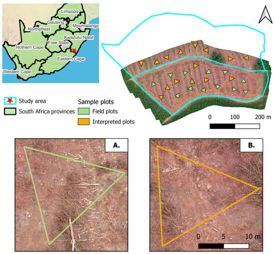
The study area is part of an industrial forest plantation located in the KwaZulu-Natal province in South Africa (
Figure 1). The complex topography of the province grants a varied and verdant climate: the area is characterized by a dry-winter humid subtropical climate, with warm summers and frequent rainfall. Winters are dry with high diurnal temperature variation, with possible light air frosts (South African Weather Service). The site, with a total surface area of 17.54 ha, is divided into two parts, which were both felled in the same period: the southern part has a surface area of 7.34 ha, whereas the northern part is larger, with a surface area of 10.24 ha.
The species planted in the study area was Mexican weeping pine (Pinus patula Schiede ex Schltdl. & Cham.), hereafter identified as pine. The harvesting operations were performed during February 2023, when the timber was mechanically felled by a harvesting machine and then extracted and transported by a forwarder to the depot. The felling machine used was a Tigercat LH822D equipped with a Log Max 7000XT head using the cut-to-length (CTL) technique, while the forwarder used was a Tigercat 1075C.
To better understand and inspect the area, the whole site was flown using a DJI Mavic Air 2S at a fixed flying altitude of 73 m, with 80% forward and 70% lateral overlap. The flight was performed in scattered-cloud-cover conditions, with the acquisition of 335 images to cover the area, resulting in a ground resolution of 2 cm/pixel. The images were handled by a Structure-from-Motion (SfM) technique using Agisoft Metashape® and combined to reconstruct the point cloud of the area. This was filtered and used to derive an orthomosaic of the study area at high resolution (2.5 cm/pixel).
2.2. Residue Data: Sampling Design and Mass Estimation
The field measurements used to estimate the mass of the harvesting residues were first carried out in March 2023 in the southern part of the site, after the majority of the forwarding operations had been completed, and before the site was burnt, therefore disposing of the residual woody material, and replanted at the end of October in the same year. Burning residues is a common management strategy widely spread in productive contexts to clean up the working area from woody debris and to create a substrate useful to establish the next generation [
5].
The sampling technique adopted was a line–intercept sampling (LIS) method [
33,
34,
35] used to estimate the volumes and weights of downed woody material over completely clear-felled areas [
36,
37]. With this method, an element is sampled if a chosen line segment, i.e., a transect, intersects the element: in this case, this technique is based on the assumptions that the residues on-site are randomly spread, with a random orientation under the transect, positioned horizontally, that they are circular in shape, and that their diameters follow a normal distribution.
Following the guidelines from Rizzolo [
38], under each transect the diameter of every visible piece of woody debris was registered and classified in time lag classes (
Table A1). Each plot was composed of three transects of 20 m each and organized as a perfect triangle with random orientation [
39] (
Figure 2); the number of triangles accounted for a total of 13 plots, hereafter referred to as “field plots”. For each field plot, the positions of vertices were recorded using a GNSS system. The time-lag division of woody material refers to the time required (in hours) for their moisture condition to fluctuate; large woody debris, for example, will inherently take longer to dry out than finer material. According to this division, material finer than 76 mm in diameter is classed as fine woody debris (FWD) and larger material as coarse woody debris (CWD). For material falling in the 1000 h+ class, i.e., with a diameter larger than 203 mm, the length of the element was also registered.
Furthermore, 14 additional plots were added across the area (using visual inspection and photointerpretation of the orthomosaic in QGIS) to increase the information available for the training of the model. These are hereafter named the “interpreted plots”, of which 8 were positioned in the northern part of the compartment. For each interpreted plot, the sampling design was similar to that performed for the field plots: the plot corresponded to a perfect triangle with sides of 20 m and residues were sampled and digitized over the transects. The diameter for each piece was recorded and sorted into classes according to
Table A1. In particular, considering the resolution of the orthomosaic (2.5 cm/pixel), it was possible to record residues with a diameter of that dimension or higher.
The residue quantity estimation (Mg·ha
−1) was performed for all categories of residue: for the 1 h, 10 h, 100 h, and 1000 h classes, Brown’s formula was used [
36,
37], as described in Equation (1). Whereas for bigger elements, i.e., those falling in the 1000 h+ class, the estimator was computed using the Woodall formula [
37], expressed in Equation (3),
where: 1.234 is a computational constant to convert the volume to m3/ha; n is the number of elements for each class; d is the average diameter for the class; c is the corrected slope (Equation (2)); a is the correction coefficient for the position of the elements, equal to 1.13 for FWD and equal to 1 for CWD; SG is the specific gravity of the wood, in this case an average value of 0.575 was adopted (575 kg m−3) [40]; L is the length of the sampling line(s); kdecay is the decay coefficient, as described in [37]–in this case kdecay = 1, since the material was freshly cut; 10,000 is the number of square meters in 1 ha; yi is the volume for a single CWD piece; and li is the length of the piece.
2.3. Satellite Data and Interferometric Processing
The Sentinel-1 mission included a constellation of two synchronous satellites (currently only one is still operating properly), equipped with a C-band synthetic aperture radar (SAR), enabling it to obtain acquisitions regardless of the weather. For this study, 4 dual-polarization Sentinel-1 SAR C-band acquisitions were downloaded from the Alaska Satellite Facility (Copernicus Sentinel data 2023, processed by ESA). The images were acquired in the interferometric wide swath mode, provided as single-look complex (SLC) data with a 250 km swath at a 5 m by 20 m spatial resolution, and captured in three sub-swaths using Terrain Observation with Progressive Scans SAR (TOPSAR).
In order to measure the changes in the surface, images were acquired not only from slightly different positions (i.e., separated by a spatial baseline), but also at different times (i.e., using a temporal baseline), a technique denoted as Differential SAR Interferometry (DInSAR). In this case, a reference image (“master”) was selected (in our case, 12 April 2023) to compare all the following changes, with the others defined as the “slave” images (6 May 2023, 17 July 2023, and 9 October 2023) (
Figure 3).
2.4. Pre-Processing of the Satellite Images
The SAR images were first processed using the Sentinel Application Platform (SNAP) from ESA (ESA Copernicus Hub). First of all, the images were inspected, and the first sub-swath was selected, as it alone contained the study area. Moreover, among the two polarizations (VH and VV), the proposed methodology relied only on the VV-polarization, since it has been proven to be more sensitive to surface moisture [
41,
42], whereas the cross-polarization signal is more sensitive to changes in the geometry and physical properties, such as the roughness [
43,
44].
The main steps of the following methodology are summarized in
Figure 4. To better fulfill the aims of this research, the images were coupled in short- (April–May), medium- (April–July) and long-term (April–October) periods. For each pair of SLC-IW single-polarization images, three explanatory variables were derived: the phase, the amplitude, and the coherence using the interferometric approach, and the intensity of the signal expressing the backscatter. The coherence provides a measure of the similarity for each pixel ranging from 0 to 1, where 0 indicates that change did happen and 1 that no change has happened. First, the images were co-registered using the S-1 TOPS co-registration process to ensure the images were aligned; their orbits were then corrected to obtain a higher location accuracy and stacked. Then, the complex interferogram was computed as a Hermitian product and the topographic phase was removed to obtain values representative for ground changes. The interferogram was multi-looked (number of looks = 3) and Goldstein phase-filtered (coherence threshold = 0.4) to enhance the coherence estimation and reduce the phase noise. After this, the DInSAR phase (∆φ), amplitude, and coherence images were geocoded and exported.
To compute the backscatter, the VV-polarized images were handled individually. After orbit and radiometric correction (using the ‘Apply Precise Orbit’ and ‘Radiometric Calibration’ commands), the images underwent multi-looking (number of looks = 3) and speckle filtering (sigma = 0.9). The images were terrain-corrected and exported as γ0 images describing the backscatter coefficient normalized by the illuminated area projected into the look direction.
2.5. Feature Extraction and the Prediction Model for Residue Mass Estimation
The following steps in the elaboration were performed using R [
45] and the RStudio environment (R version 4.4.1; RStudio 2024.04.2+764 “Chocolate Cosmos”). After the pre-processing, the ∆φ, amplitude, coherence, and γ
0 images were stacked together and handled as a raster, using the
terra package [
46]. The plots were paired with the mean quantity value obtained by averaging the estimations from their sample lines. The shapefile containing this information was used to extract the mean value from the stacked backscatter and then converted to a data frame.
The data frame was used to feed two models: a generalized linear model (GLM) and a Random Forest model (RF). These models were selected because of the underlying assumptions upon which they work, GLM being a parametric model and RF being a non-parametric model. The main distinction between the chosen categories is that parametric models are faster to use, but they imply stronger assumptions about the data distribution, whereas non-parametric models are more flexible but are computationally intractable for larger datasets [
47]. In the first case, the application of a linear model also had the intention to find possible correlations between the variables and to underline possibly significant variables available in the data frame. Specifically, in the case of GLM, all variables were used to feed the model. The RF model used is a machine learning algorithm built from the R package
randomForest [
48], with a forest size of 500 trees (
ntree = 500); all variables were used to initially feed the model, and the split decision parameter (
mtry) was adequately set. For both models the training and testing was performed using a leave-one-out cross-validation (LOOCV) procedure. The RF model was then iteratively adjusted by progressively excluding the variables that reported a negative importance score.
2.6. Coherence Difference Analysis
To better gain insights into the results, a separate analysis was performed to consider the coherence values, comparing each image pair and computing the differences between the pairings. The coherence (ϒ) values are calculated at pixel level and range from 0 to 1; a value of 1 indicates no alteration in the scattering properties between images [
49]. However, when the observed surface changes, the complex backscatter is impacted, causing a decrease in coherence, which is known as decorrelation. This approach moves on from previously established coherence difference analysis (CDA) methods [
50] but still follows the same purpose, i.e., to define and to investigate the source of decorrelation. Consistent with [
51], interferometric coherence is affected by three main factors of decorrelation: radar thermal noise decorrelation (ϒ
N), geometric decorrelation (ϒ
G), and temporal decorrelation (ϒ
T). Considering that all the images were acquired by the same antenna, it is reasonable to assume that the variation in thermal noise between the images will not influence the coherence decorrelation [
49]. The geometric decorrelation, on the other hand, is highly influenced by the perpendicular baseline; if this parameter is greater than the critical value, then ϒ
G becomes 0, causing the maximum decorrelation [
52]. Finally, the temporal decorrelation is the one that would contribute the most, since the loss in coherence is mainly due to changes in the object’s properties (i.e., the geometric structure and dielectric properties). In this case, the coherence difference analysis assumed that the presence of harvesting residues in clear-felled areas would be less stable over time than the surrounding solid soil (due to decomposition processes, residue pile volumes gradually collapsing to a solid ground layer, etc.). Hence, the residues would decorrelate more (measured as a decreasing coherence) as time passes. The variation in the dielectric constant was assumed to be lower for the surrounding clear-cut plantation, and hence present only smaller changes in the backscatter between the SAR images.
2.7. Validation Assessment
Both models were validated by using the field plots as a reference and comparing the predicted values against the estimates obtained through volume calculation. In this case, two indicators were considered: the squared Pearson index (R2) to evaluate the correlation between the field values and the predicted values, and the Root Mean Squared Error (RMSE) to assess the model’ performance. At the end, the model was used to predict the residues’ mass distribution throughout the study site.
To further evaluate the goodness of the estimations and mapping produced for the residues, the field plots were also visually inspected, and the diameter of the material was registered, with the residue’s mass computed. After this, the bias and RMSE were computed.
4. Discussion
This paper aimed to evaluate the possibility of using SAR data techniques (InSAR and DInSAR) to quantify the mass of harvesting residues left in clear-felled areas. To achieve such an aim, an innovative approach was offered by comparing two prediction models (GLM and RF) and evaluating their goodness-of-fit (R2), RMSE, and bias.
Considering the coherence difference analysis, the assumptions implied a higher decorrelation for the residues compared to the surrounding solid soil, where the variation in the dielectric constant values would present only smaller changes in the backscatter between the SAR images. In this case, where the main source of decorrelation is tributed at both the temporal and spatial baselines, the difference in the perpendicular baselines ranged from 54 to 117 m, which is a bit large for the sensitivity that was aimed for, since the objective was to observe small differences within fractions of the wavelength considered (i.e., ~4 cm for the C-band). Nevertheless, the range of values found is well below the critical baseline reported in the literature (e.g., [
53,
54]). Nevertheless, the loss of coherence was useful in our predictions.
In the short term, the coherence exhibits higher values inside the harvesting area, with more variations outside the perimeter, where the trees are still standing, as also reported by Akbari et al. [
55], whereas the coherence gradually decreases with time, resulting in values close to zero. Variations in the coherence throughout the time of observation might also be due to precipitation events before the acquisition of each satellite image (
Figure A2), and, more importantly, before acquisition of the master image. Therefore, the fluctuation in coherence values in the short term are likely due to changes in the dielectric constant happening in the days right before the image acquisition (although in between images there were periods of relatively stable weather patches), rather than due to changes in volume scattering. Changes in the surrounding trees are more likely related to fluctuations in the crown water content, due to the SAR operating at C-band [
56]. These assumptions are also supported by the ∆φ images (
Figure 5), where greater differences are shown from the first interferogram and the coherence differences, where lower changes are noticed outside the logged area (
Figure 6C,E). Some of these findings were also noted when developing the linear prediction models, where the relation and contribution of the various variables were studied. For example, in the GLM model, the variables with the highest significance came from the short-period interferogram (i.e., the April–May interferogram), which also exhibits a higher variation in the coherence values. On the other hand, the RF model prefers the phase difference between April and May, but also the amplitude from April-October (long term) and the γ
0 from July.
The magnitude of the residue masses estimated from the field survey are comparable with the values available in the literature for the species considered [
39,
57]. The higher residue mass values of the interpreted plots (+51% compared to the field plots) can be due to the influence of several factors. First of all, due to the interpretation and visual inspection of the logging area by means of aerial photogrammetry: although available with a fairly high resolution (2.5 cm/pixel), the orthomosaic used for the visual assessment of the residues still did not allow for the inspection and registration of smaller woody material with diameters less than 3 cm (i.e., the 1 h and 10 h classes). This could be reflected in the average quantities per plot, which are higher in the interpreted plots compared to the field ones. Moreover, whereas the field survey also considered stumps, the visual inspections did not, therefore further reducing the estimated amount of the CWD material. A similar issue can be found also in [
30], although using a different system for manual annotation. Secondly, the presence of residue piles in the area does not allow for an optimal visual annotation of the material from QGIS, since it would be possible to register only the diameter of the elements on the very top of the pile, whereas with the field survey some material from the deeper layer can also be registered. Therefore, the volumes or masses considered result in different values, also for the same plots, as exposed by the bias evaluation (−0.05 Mg and 0.14 Mg, for the CWD and FWD+CWD material considered).
Nevertheless, there are different factors and limitations to consider for this study and the proposed methodology. The main principle of the DInSAR technique adopted is that it allows for the retrieval of any changes on the surface of the area investigated, through the scatter of the beam signal; the rougher the object, the more scatter it should produce.
Overall, this study investigated only the use of VV-polarization acquisitions, based on the previous literature, considering any major detectable changes due to moisture variation in the residues and piles rather than in their geometry and structural properties. Considering the object of the investigation, the harvesting residues, although not individually detectable using the SAR pixel size (10 m × 10 m), can be addressed in piles, offering a large (on average, 5 m wide and 1.5 m tall at maximum), complex, and rough target when performing this kind of research. However, obtaining precise information on the pile masses and volumes is still challenging, both with field measurements and remote sensing-based techniques [
57,
58,
59].
Regarding the study area, the site presented homogeneous characteristics, being a pine plantation with a moderate slope where forest machines could work [
60] and with the residual material distributed in an ordered scheme, following the work system. Still, some of the features of the area could have helped to overestimate or underestimate the actual biomass left.
The use of C-band is preferred in scenarios where low volumes of biomass need to be estimated (e.g., in clear cuttings) [
61] but they are still subject to a relatively small saturation threshold, of 60–70 Mg/ha [
32,
62]. Specific to the methodology proposed, the analysis of coherence provided insightful information about the signal scattering and its changes throughout the monitored period. Although minimized, different sources of decorrelation might have still played a role in the obtained results, especially the geometric decorrelation. Moreover, to properly address the volume scattering, the proposed methodology featured also the backscatter signals, γ
0, but saw limited contribution from the majority of them (
Figure A1). In this case, the possible addition of VH-polarization backscatter could add complexity to the response, delivering a more comprehensive output.
An issue more related to the prediction models is the number of available plots used to feed the model and its design: a higher number of observations would have probably increased the R
2 of the results and their robustness, for both the GLM and RF models. In fact, both models can be easily exposed to a dataset with a limited number of observations, in particular the RF model [
63]. Nevertheless, the models’ outcomes are inherently constrained by the aforementioned limitations, as they represent the final stage of the analysis.
5. Conclusions
This study evaluated the possibility for SAR data to predict the quantity of harvesting residues over clear-felled areas, performed over a study area of a pine plantation in South Africa. The models’ predictions provided results with an R2 index of 0.47 and 0.13 for GLM and RF, respectively, when using all the plots, and 0.23 and 0.006 when using only the field plots. The RMSE stabilized between 0.20–0.28 Mg. Overall, the bias regarding the interpretation of the woody material ranged between −0.05 and 0.14 Mg. Nevertheless, we can positively affirm that, even at this stage and with the limitations listed above, it is possible to derive useful indications about the mass of harvesting residues from SAR data handled with InSAR and DInSAR techniques.
This information could be suitable for forest owners and managers interested in the possible retrieval of material to convoy to bioenergy-producing plants, or to provide an indirect estimation of possible C-stock in woody material to help industrial companies account for carbon or reduce their impact on biogeochemical cycles and nutrient fluxes in the re-establishment of timber plantations and the use of fertilizers.
Future research should investigate alternative SAR techniques and the potential integration of other remote sensing technologies, such as LiDAR, and the application of models to different forest types. Moreover, it could be interesting to explore the possibility of conducting different observations at different sites at the same time to address local variability between sites and/or species.