Deep Learning Autoencoders for Fast Fourier Transform-Based Clustering and Temporal Damage Evolution in Acoustic Emission Data from Composite Materials

2. Materials and Methods

This section outlines the methodology employed in this study (Figure 1), detailing the steps taken from data acquisition to the analysis of damage evolution in CFRP structures. It begins with an overview of the experimental setup and the procedures used for data collection. The subsequent phases cover the signal pre-processing and transformation of AE data from the time domain to the frequency domain using FFT, followed by the application of deep autoencoder networks for learning compact representations of the processed signals. The latent space representations obtained from the autoencoder are then subjected to unsupervised clustering to identify distinct damage states. Visualization techniques are employed to interpret the results, and finally, Markov chain analysis is used to model the temporal evolution of damage. Each stage of the methodology contributes to a comprehensive framework for detecting and monitoring damage progression in CFRP structures.

2.1. Experimental Setup

CFRP coupons manufactured using the resin infusion process were used in mechanical tensile and three-point flexural tests that were carried out as part of the Horizon 2020 Carbo4Power project. Collection of the AE data utilized for initial analysis and as input for model creation was completed through monitoring during the mechanical tests. Specific focus was placed upon CFRP, which have been employed for the reinforcing spar during WTB manufacturing. The reinforcing spar is the main load-bearing component of the WTB. The intended role of the material guided the selection of mechanical testing, ensuring that the applied loading conditions closely replicate those expected in real-world applications. From the AE data captured during tensile and flexural testing, it was possible to establish the relationship between AE response and associated damage mechanisms developing from the healthy condition of the material up to its final failure.

Tensile testing was performed using an electro-mechanical testing machine manufactured by Zwick Roell, model 1484, with a 200 kN load cell. The extensometer length was set to 10 mm, and the crosshead movement speed was set to 2 mm/min. Test coupons with dimensions 250 mm long by 25 mm wide were used for the tensile tests, with a thickness range of 1.03–1.33 mm. These had a laminated layered structure with fiber direction of [0/45/QRS/−45/90], where the QRS are Quantum Resistive Sensors in the shape of wires with a diameter comparable to that of the fibers. QRS were internally positioned, interlaminar sensors for direct measurement of strain, temperature, and humidity developed as part of the Carbo4Power project. End-tabs were used to allow for the proper application of the grip force during loading. Three-point bending testing was carried out using a Dartec Universal Mechanical Testing Machine, with a 50 kN load cell and a crosshead movement speed of 1 mm/min. Test coupons with dimensions 150 mm long by 25 mm wide and a thickness range of 1.15–1.32 mm. Again, these example coupons were of a layered laminated structure, with a layup of [0/QRS/45/−45/90]; due to the nature of the specific mechanical testing, no end tabs were required.

2.2. Data Collection

The data collection was performed using two R50αa narrow band resonant piezoelectric sensors manufactured by Physical Acoustics Corporation. The operational frequency range of the R50α sensors is from 150 kHz to 500 kHz, such that the frequency response of the sensor is optimized for detection in this range. The sensors were mounted on the same side of the samples at each end using Araldite two-component epoxy adhesive, as illustrated in Figure 2.

The outputs of the sensors were amplified in two stages, a 40 dB pre-amplification followed by another 9 dB using a bespoke 4-channel variable gain amplifier manufactured by Feldman Enterprises Ltd. The amplified signal was filtered at 500 kHz for anti-aliasing purposes and was digitized using a 4-channel 16-bit National Instrument 9223 Compact Data Acquisition (NI-cDAQ) module. The NI-cDAQ module was connected to a very small Intel Next Unit of Computing (NUC) computer using a cDAQ-9171 via a USB port. The data acquisition was performed using bespoke software written in MATLAB R2023b and developed in-house using NI-DAQmx, which was hosted on the NUC computer. The recorded datasets were captured at 1 MSamples/s per channel periodically for 5 s with a 1 s delay between each recording, collecting data from 9 specimens for analysis. Figure 3 illustrates a raw dataset recorded from a sample under 3-point flexural testing up to failure.

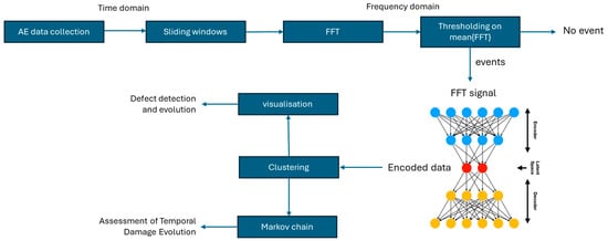
2.3. Signal Pre-Processing and FFT Transformation for Time-to-Frequency Domain Analysis

In the first phase of the methodology (Figure 4), noise is minimized through the usage of bandpass filtering in the preamplifier (20–1200 kHz) as well as the usage of thresholding of the signal. Additionally, offset has been corrected through DC offset correction, lessening the mean of the signal from itself to remove the effects of electronics. The denoised AE signals are then transformed into the frequency domain using FFT. This transformation is essential for revealing key frequency components associated with different types of damage that may not be as evident in the time domain. A sliding window approach is applied with a window length of 200 samples and a step size of 100 samples, ensuring that overlapping segments were analyzed for better temporal resolution.

After applying the FFT to each windowed signal, the mean FFT is computed to create a representative frequency spectrum. Each transformation yields 100 frequency components, determined by the sampling rate and window length. To retain only the most relevant frequency components and suppress noise, a thresholding technique is used. The threshold for frequency-domain event selection was determined through an empirical sensitivity analysis using the statistical properties of the noise level in the dataset. The analysis considered the mean and standard deviation of the background noise, along with percentile-based thresholds, to establish a threshold that effectively filtered out insignificant fluctuations while preserving relevant AE events. The threshold selection was refined within the range [0.0050–0.0126], corresponding to the 99.9th to 99.99th percentiles of the signal. A grid search was performed within this range, starting from 0.0050 with a step size of 0.001, evaluating the separation between noise and meaningful AE events at each step. The selected threshold (0.01) ensures that only the most critical frequencies, those indicating potential damage, are passed on to the next phase of the analysis. Specifically, frequency components exceeding the 0.01 threshold in the mean FFT spectrum are retained, while lower-amplitude components are discarded. This reduces data dimensionality and ensures that only the most informative frequencies are passed to the autoencoder. By emphasizing significant signals and suppressing noise, the thresholding process enhances damage detection accuracy, making the subsequent analysis more robust and focused on critical frequency behaviors over time. As a result of this process, a total of 2,099,313 AE events were identified and selected for further analysis from the data collected across all 9 specimens, with each event represented by a time segment of 200 time samples and its corresponding frequency representation consisting of 100 frequency components.

2.4. Learning Compact Representations Through Deep Autoencoder Networks

The training of the autoencoder represents a critical phase in the overall methodology, where the model learns to compress the input data into a lower-dimensional latent space and then reconstruct it with minimal loss of information [23]. The input data to the autoencoder consists of the FFT values, after the threshold implementation, carefully filtered to retain only the most significant frequency components. The primary objective of training the autoencoder is to learn a compressed representation of these data in the latent space while minimizing the reconstruction error between the input and output.

The autoencoder architecture consists of two main components: the encoder and the decoder. The encoder is responsible for mapping the high-dimensional input data to a lower-dimensional latent space. During this process, the encoder learns to identify key features in the data that are essential for representing the underlying structure of the signals, effectively reducing the dimensionality of the input. The dimensionality of the latent space is determined through hyperparameter tuning, ensuring that it is compact enough to be efficient, yet large enough to retain critical information about the damage-related frequency components. Once the data have been compressed into the latent space, the decoder is tasked with reconstructing the original input data from this lower-dimensional representation. The decoder mirrors the encoder, gradually upscaling the compressed data back into its original high-dimensional form. The success of this reconstruction is measured by the reconstruction error, which quantifies the difference between the original input and the reconstructed output. The goal of training is to minimize this error, ensuring that the latent space captures the most informative features of the data with minimal loss of fidelity.

The training process involves iteratively adjusting the weights of the encoder and decoder through backpropagation. The autoencoder is trained using mean squared error (MSE) as the loss function, which measures the average squared differences between the input and reconstructed output. By minimizing MSE, the autoencoder learns to effectively encode the “thresholded” FFT data in a way that preserves its key characteristics while discarding irrelevant noise and redundant information. During the training process, Bayesian optimization was employed to fine-tune the hyperparameters of the autoencoder. This optimization process explored various configurations, including the size of the latent space, the regularization terms, and the number of training epochs, to find the optimal settings that resulted in the lowest reconstruction error. The use of L2 weight regularization and sparsity constraints ensured that the autoencoder did not overfit the training data, promoting a more generalized model that performs well on unseen data.

The autoencoder’s architecture is designed with several key hyperparameters that control its performance. These included the following: (i) L2 weight regularization to prevent overfitting by penalizing large weights; (ii) sparsity regularization to enforce a constraint that encourages the latent space to have a sparse representation, meaning that only a few neurons are activated for any given input; (iii) sparsity proportion, which controlled the degree of sparsity in the latent representation; (iv) encoding dimension, which determined the size of the latent space and, therefore, the degree of compression; and (v) maximum number of epochs, which defined the number of training iterations. The optimal values of these hyperparameters were identified using Bayesian optimization, which efficiently searched for the best combination of parameters by balancing exploration and exploitation of the hyperparameter space. This process minimized the reconstruction error and ensured that the autoencoder learned an optimal latent space representation of the normalized FFT data.

The autoencoder’s performance has been evaluated by assessing the ability to accurately reconstruct the original input data from the latent space. The reconstruction error, measured in terms of MSE between the original and reconstructed signals, served as the primary metric for evaluating the model’s performance. The reconstructed signal

\hat{X_{i}}

for each window

i

was compared to the original normalized FFT data

X_{i}^{n o r m}

, and the reconstruction error was calculated as follows:

$M S E = \frac{1}{n} \sum_{i = 1}^{n} {(X_{i}^{n o r m} - \hat{X_{i}})}^{2}$

(1)

where n is the number of frequency components in each FFT vector. A low reconstruction error indicates that the autoencoder has effectively learned to compress and reconstruct the key features of the data. To ensure model generalization, we applied a Leave-One-Experiment-Out (LOEO) cross-validation approach, training on 8 out of 9 experiments while using the remaining one for testing, repeating this process 9 times. Since the duration of each experiment varies, the number of AE events in the training and testing sets was not fixed. However, on average, approximately 90% of the total 2,099,313 AE events were used for training, while the remaining 10% were allocated for testing in each cross-validation fold. This ensured that the model was trained on a diverse set of AE signals while being evaluated on previously unseen data, improving its generalization ability and robustness. In addition to the quantitative evaluation, qualitative assessment was also performed by visualizing the reconstructed signals alongside the original FFT data. This visual comparison helped to ensure that the shape of the FFT, which was critical for clustering, has been preserved during the dimensionality reduction process.

2.5. Clustering in the Latent Space

Once the autoencoder has performed the dimensionality reduction, the next important step was clustering the latent representations of the AE data. Clustering helped reveal hidden patterns in the latent space, which can correspond to different damage-related events. This section explained the clustering methodology, evaluated its performance, and provided a theoretical background along with result visualizations. The latent space generated by the autoencoder reduced the normalized FFT-transformed AE data into a lower-dimensional space that preserved the most critical features. Each point in the latent space corresponded to a windowed segment of the AE signal, representing the key signal characteristics captured by the autoencoder.

Z \in R^{n \times d}

corresponds to the matrix of the encoded features, where

n

was the number of AE windows and

d

was the dimensionality of the latent space (optimized during autoencoder training). The goal of clustering in this latent space is to group data points

Z_{i} \in R^{d}

into clusters, where each cluster potentially represents a distinct damage event or state. We utilized then k-means clustering, as an unsupervised learning algorithm, to partition the data into

k

clusters based on the latent representations of AE data. The k-means algorithm iteratively assigned each data point

Z_{i}

to one of the

k

clusters, represented by centroids

C_{j} \in R^{d}

, to minimize the within-cluster sum of squares (WCSS), which is defined as follows:

$W C S S = \sum_{j = 1}^{k} \sum_{Z_{i} \in C_{j}} {| | Z_{i} - C_{j} | |}^{2}$

(2)

The algorithm proceeded in two steps: (1) Assignment Step: Assign each data point to the nearest cluster centroid and (2) Update Step: Update the centroids as the mean of the points in their respective clusters. To ensure an optimal choice for the number of clusters k, we evaluated clustering performance using the Silhouette Score, a metric that quantifies how well-separated the clusters are. We tested different values of k within a predefined range (from 2 to 5) and selected the one that maximized the mean Silhouette Score, indicating the best balance between cluster cohesion and separation. This approach ensured that the latent representations of AE signals were grouped into distinct damage-related states while minimizing overlap between clusters. Furthermore, in order to improve initialization, we employed k-means [24]. This method selected initial centroids in a way that spread them out, reducing the likelihood of poor clustering. The first centroid,

C_{1}

, was selected randomly, and each subsequent centroid was chosen based on the distance from the nearest previously selected centroid. The probability of the choosing point

Z_{i}

is expressed as follows:

$P (Z_{i}) = \frac{{D (Z_{i})}^{2}}{\sum_{j} D {(Z_{j})}^{2}}$

(3)

where $D (Z_{i})$ is the distance to the nearest centroid already chosen. This initialization improved the likelihood of finding globally optimal clustering. After determining the optimal clusters, we were able to classify new AE signals. For a new set of encoded features $Z_{n e w}$ , each data point was assigned to the closest cluster centroid from the original clustering.

$\hat{C (i)} = \arg m i n | | Z_{n e w, i} - C_{j} | |$

(4)

where $Z_{n e w, i}$ is the encoded feature for a new data point and $C_{j}$ is the centroid of the $j$ -th cluster from the original k-means model.

2.6. Visualization

After clustering latent space representations, it was crucial to visualize clusters to understand how they group and relate to time-series data. We plotted the mean frequency content of each signal over time and color-coded the points according to their cluster. Visualization provided insights into the structure and evolution of clusters, allowing us to assess the characteristics of AE signals in relation to material damage events. The mean frequency content

X_{i}

is calculated as follows:

$X_{i} = \frac{1}{n} \sum_{j = 1}^{n} F F T_{i j}$

(5)

where n is the number of frequency components. The points are then plotted against time $t$ , with different colors representing clusters. In addition to the latent space clusters, we plotted the accumulated mean frequency for each cluster over time. The following expression is the cumulative sum of the mean frequency content for signals within each cluster:

$A c c_{c} (t) = \sum_{k = 1}^{t} X_{i}$

(6)

This time-dependent view revealed frequency trends for each cluster, showing signal characteristics at different stages of damage. In order to understand the spectral characteristics of each cluster, we computed the mean frequency content

μ_{κ}

and its standard deviation

σ_{κ}

$μ_{κ} = \frac{1}{| C_{k} |} \sum_{X_{i} \in C_{k}} X_{i}$

(7)

$σ_{κ} = \sqrt{\frac{1}{| C_{k} |} \sum_{X_{i \in C_{k}}} {(X_{i} - μ_{κ})}^{2}}$

(8)

where $C_{k}$ is the set of signals in cluster $k .$

2.7. Temporal Damage Evolution Using Markov Chain Analysis

To analyze the temporal dynamics of clusters, we modeled transitions between clusters using a Markov chain. This approach allowed us to capture the frequency and likelihood of AE signals transitioning between different clusters over time, providing insights into the evolution of damage states within the monitored structure. Each cluster represents a specific stage or type of damage, and the transitions between them help us understand how damage progresses, stabilizes, or regresses. This captured how frequently AE signals transitioned between clusters, corresponding to different damage stages. The transition matrix

P

is expressed as follows:

$P_{i j} = \frac{T_{i j}}{Σ_{κ} Τ_{ι κ}}$

(9)

where $T_{i j}$ is the number of transitions from cluster $i$ to $j$ and $Σ_{κ} Τ_{ι κ}$ is the total number of transitions from cluster i to any other cluster, ensuring that the probabilities in each row of the matrix sum to 1.

This formulation allows us to calculate the relative likelihood of transitioning between clusters, effectively capturing the progression from one damage state to another, as well as the likelihood of remaining in the same state (self-transitions). The higher the value of $P_{i j}$ , the more likely it is that an AE signal moves from state i to state j, while low values indicate rare transitions or relatively stable states. The transition matrix is visualized as a state transition diagram. The state transition diagram is a graphical representation of the clusters and the transitions between them. Each node in the diagram represents a cluster, while the arrows between nodes indicate the direction and magnitude of transitions between states. The thickness of each arrow is proportional to the transition probability between clusters, with thicker arrows indicating more frequent transitions. Self-transitions are also represented by loops at each node, indicating the probability that a signal remains in the same cluster (damage state) over time. This diagram provides a clear view of the overall flow between different damage stages, allowing for an easy interpretation of how the system evolves.

The Markov chain analysis offers valuable insights into the temporal progression of damage in CFRP structures. By examining the transition probabilities, we can make several important observations:

Clusters with high self-transition probabilities (i.e., large values of $P_{i j}$ ) are considered stable states. These clusters represent damage stages that persist for longer periods before transitioning to another state. For instance, if the probability of staying within Cluster 1 is high, it suggests that this stage of damage is more prolonged or stable.
The transition probabilities between clusters $P_{i j}$ reveal how damage evolves over time. For example, a high probability of transitioning from Cluster 1 to Cluster 2 would indicate that damage is progressing from an early-stage or less severe state (Cluster 1) to a more advanced or severe stage (Cluster 2). These transitions are critical for understanding how damage accumulates and the speed at which it progresses.
The Markov chain also allows for the analysis of reversibility in damage progression. If there is a significant probability of transitioning back from Cluster 2 to Cluster 1, this could suggest that certain damage processes may stabilize or revert under certain conditions, such as cyclical loads. This could be indicative of periods where the structure is subjected to temporary stress without permanent damage progression.

By modeling the system as a Markov chain, we can use the transition probabilities to forecast future states of the system. For instance, if there is a high probability of transitioning from a stable damage state to a more critical one, maintenance activities can be scheduled pre-emptively, reducing the risk of unexpected failures.

2.8. Assignment of Frequency Ranges for Damage Mechanisms

For the assessment of damage using the frequency components contained within a given AE event signal, it is important that the identified peaks and features can be properly attributed to their respective sources and hence, related damage mechanisms. The relationship between energy and frequency is well established, with observed damage mechanisms within an FRP also generating signals with distinctive energy content, which is dependent on the relative interfacial strength. When assessing damage mechanisms, attempting to characterize them using a specific frequency value can result in significant inaccuracies, particularly since the propagation of the wave with increasing distance from the source will result in signal attenuation but also frequency dispersion. Hence, assigning ranges to the associated frequencies from observations of the transformed spectra can contribute to the correct identification of the damage mechanism affecting a particular FRP component during damage initiation and subsequent evolution. Accurately assigning the frequency ranges associated with different damage mechanisms will allow the effective damage mechanism identification and monitoring of damage initiation and evolution in FRP components.

One way of achieving this is through the evaluation of the peak observed frequency for an extracted AE event ([25,26,27]). In previous studies published on the subject, commercial software with automated analysis has been commonly used. Herewith, we have employed a custom-built AE system and associated software. As this only relies on fairly simple DSP approaches, the process can be executed with high sensitivity, accuracy, and robustness in a time-efficient manner, with required operations completed post-acquisition. When assessing this in a way that allows the relative density of the extracted peak frequencies to be obtained, clear bands can be observed within the analyzed signals, considering both frequency versus elapsed time and measured magnitude.

The extraction of peak frequency allows for the assessment of the primary contributing phase within the captured waveform. Hence, information on the dominant damage mode for a given identified AE event can be obtained. Knowing the usual damage progression within the tensile loading of the test coupons also assists in the assignment of damage modes to the bands, which can be seen to be present. Based on the damage mechanisms in FRPs, five distinct bands are expected to arise, one for each of the primary damage mechanisms.

Matrix cracking has been assigned to the lower frequency range of 100–200 kHz. This extended range can be attributed to different directional behavior associated with matrix cracking within the samples tested, not only in relation to the fiber direction in relation to the individual laminates, which can give rise to both longitudinal and transverse matrix cracking. Also, the through-thickness matrix cracking, with cracks propagating perpendicular to the general plane of the material. The frequency ranges identified were observed across all samples tested, for both tensile and flexural testing. Hence, these frequency ranges can be employed for the evaluation of damage for materials tested. However, it is noted that the exact frequency range values are also material dependent, exemplified through extensive review [22]. Hence, this approach requires a given material to be characterized before further conclusions can be made regarding damage characterization, with the intended sensor also utilized. Despite the material-specific dependencies and other factors influencing the exact frequency values for damage, as well as the challenges in directly comparing with literature, the assigned values can still be evaluated in relation to established trends observed in similar materials and setups. To support this, a targeted literature review was conducted, focusing on studies with comparable experimental conditions. The corresponding values are presented in Figure 5, which illustrates variations in reported frequency bands for matrix cracking, delamination, debonding, fiber breakage, and fiber pull-out.

While the selected studies prioritize similarity in material composition and AE setups, differences in mechanical testing methodologies and DSP techniques contribute to the observed variations. Nevertheless, Figure 5 highlights a strong consistency in the relative positioning of damage modes within the established frequency ranges, reinforcing the validity of the assigned frequency bands in this study.

3. Results

This section presents the results of our analysis of AE signals using frequency-domain transformations, autoencoder-based representation learning, and clustering techniques. Additionally, we present the outcomes of applying Markov chain analysis to model the temporal evolution of damage, offering insights into the progression of damage states over time.

3.1. Damage Detection

Figure 6 illustrates the peak frequency assessment of a tensile-tested CFRP sample coupon by plotting (a) time vs. peak frequency and (b) magnitude vs. peak frequency. The observed clustering of frequency values into distinct bands aligns with expected damage mechanisms in CFRP materials. As outlined in Table 1, different damage modes exhibit characteristic frequency ranges, with matrix cracking occurring in the 100–200 kHz range, delamination in the 200–250 kHz range, and more severe damage modes such as fiber breakage and fiber pullout appearing at higher frequencies (above 325 kHz). The observed frequency bands support the idea that AE-based frequency analysis can be effectively used to classify different damage types. In both subplots, the majority of the detected peak frequencies fall within the anticipated damage mode ranges, suggesting a strong correlation between the AE events and specific failure mechanisms. Peak frequency values below 100 kHz have been designated as anomalous, likely resulting from noise or the misidentification of an AE event as damage. These signals are typically associated with low amplitude. Across all datasets, only a few such cases were observed, with no discernible trend. Beyond this, these events tend to be of lower intensity and, in some cases, are entirely absent. Given these factors, no definitive conclusion can be drawn regarding their origin. However, they are most likely due to noise misclassification or damage to the pure resin system used for the end-tabbing of the test coupons. In subplot (b), plotting magnitude versus peak frequency further reinforces the differentiation between meaningful AE events and noise. The intensity of AE events is generally higher in the mid-to-upper frequency ranges, corresponding to damage modes such as delamination and fiber breakage. This distribution confirms the effectiveness of frequency-based AE analysis for detecting and characterizing structural damage in CFRP materials.

Figure 7 presents a comparative view of AE signals in both the time and frequency domains, demonstrating cases with detected AE events (subplots a, b, and c) and without detected AE events (subplots d). While the time-domain signals (top row) provide some information about the AE events, they often contain complex oscillations that may overlap with noise or other irrelevant fluctuations. As a result, they may not clearly differentiate between significant events and background noise. In contrast, the frequency-domain plots (bottom row) offer much more distinct insights. In subplots (a) and (b), clear frequency spikes emerge in the FFT plots, revealing dominant frequency components that are directly tied to the detected AE events. These frequency spikes make it easier to identify and interpret the occurrence of specific damage-related phenomena. The sharp peaks in the frequency domain provide critical insights into the nature of the AE events that are less obvious in the time domain. These peaks correspond to specific vibrational modes or energy releases, which can be directly associated with the physical mechanisms causing the damage. As such, the frequency domain is much more revealing in terms of identifying and classifying different types of AE events.

Subplot (c) demonstrates how the transition to the frequency domain allows the detection of subtle but significant events that may be difficult to isolate in the time domain. In this case, the presence of dominant frequencies points to specific damage signatures, which are not as clearly discernible in the raw time-domain signals due to normal oscillations ranging between −0.005 and 0.005, making it challenging to distinguish damage-related events from background noise. This sensitivity to specific frequency components allows for much earlier and more precise detection of defects compared to time-domain-only analysis. The subplot (d), which represents a period without any detected AE event, shows how the frequency domain remains insightful even in quieter scenarios. While the time-domain signal still shows a minor fluctuation (with a peak value lower than −0.005), the frequency-domain plot reveals no significant peaks, indicating that no meaningful AE events are present. This clear distinction helps reduce false positives, as the frequency-domain analysis can filter out inconsequential noise and focus on genuine event signatures.

Figure 8 presents a frequency-domain analysis for event detection, where the signal thresholding is applied to identify significant events in a lab experiment. The plot shows the amplitude difference in the mean FFT values across multiple window indices, with the threshold set at 0.01, indicated by the red dashed line. This threshold helps distinguish between normal fluctuations in the signal and potential anomalies or events of interest.

The transition from the time domain to the frequency domain significantly enhances the detection sensitivity for damage events. In this case, the use of mean FFT analysis reveals amplitude differences across various windows, providing a clearer view of the frequency components contributing to defect events. Traditional time-domain analysis may not be able to detect these subtle changes, but frequency-domain methods allow the identification of small amplitude deviations that could be indicative of evolving damage. The chosen threshold of 0.01 acts as a critical marker to highlight significant anomalies or events. In the presented experiment, most of the data points remain below the threshold, indicating normal or less significant frequency variations. However, there are distinct peaks that surpass the threshold, signaling potential damage events. This method not only detects events but also reduces the chance of false positives by focusing on those exceeding the defined amplitude difference threshold.

3.2. Representation Learning Results

Table 2 presents the key hyperparameters and performance metrics of the trained autoencoder model, providing a detailed overview of both its structure and its effectiveness in reconstructing input data. The hyperparameters were fine-tuned using Bayesian optimization to achieve the best possible performance for feature encoding and reconstruction tasks. Figure 9 illustrates the convergence behavior of the Bayesian optimization process. The objective function values across iterations are shown, with the best objective value tracked over time. The smoothed trend highlights the overall improvement, while the final best-found solution is marked. This visualization demonstrates the optimization’s effectiveness in progressively refining the hyperparameters to minimize the objective function. The L2 Weight Regularization is set to a low value of 4.0959 × 10^−0.5, indicating that minimal regularization was needed to prevent overfitting while still maintaining the generalization capability of the model. This balance is crucial for allowing the model to effectively capture the structure of the data without excessively constraining its learning capacity.

The Sparsity Regularization (0.26843) and Sparsity Proportion (0.27307) parameters further control the sparsity of the encoded representations. These values suggest that the model is encouraged to learn compact representations by activating fewer neurons in the latent space, thus making the encoded data more concise and focused on the essential features. The encoding dimension of 76 specifies the size of the latent space, determining the number of features retained after compression. This dimensionality is sufficient for the model to effectively represent the high-dimensional input data while still significantly reducing its size. The training process was allowed to run for 293 epochs, which indicates that the model was given ample time to converge to an optimal solution, allowing it to iteratively improve its performance. The performance of the autoencoder is assessed through two key metrics. The global MSE is quite low at 0.0017259, suggesting that the model performs well in reconstructing the input data, with minimal deviation between the original and reconstructed data. This low reconstruction error demonstrates that the model is successfully capturing the key patterns in the data. Similarly, the global R-squared (R²) value of 0.94774 shows that the model explains a very high proportion (about 94.77%) of the variance in the input data. This high R² value is a strong indicator of the autoencoder’s ability to retain the most important information while compressing the data into a lower-dimensional space.

Figure 10 above shows a comparison between the original and reconstructed FFT signals for four different examples. In each subplot, the original signal (in blue) is plotted against the reconstructed signal (in red dashed lines), providing a visual indication of the autoencoder’s reconstruction accuracy. The close alignment between the original and reconstructed signals across all four examples reinforces the earlier quantitative findings, particularly the low MSEs within the range of [0.000367, 0.000518] and high R-squared (R²) values ([0.9771, 0.9822]). These plots highlight that the autoencoder effectively captures the underlying structure of the FFT signals, reproducing the peaks and amplitude variations with minimal deviation. The slight differences in some regions, particularly near higher amplitude peaks, may represent the minor reconstruction errors that contribute to the low MSE value observed. Overall, these visual results confirm the model’s capability to faithfully reconstruct the original signals, further validating its use for tasks such as feature extraction, dimensionality reduction, and defect detection in frequency-domain data. This ability to maintain the essential characteristics of the signal through reconstruction illustrates the effectiveness of the hyperparameter tuning and model architecture discussed earlier.

3.3. Clustering Results and Visualization

Table 3 shows the clustering results based on the analysis of silhouette scores. This table compares the performance of different clustering configurations, where the silhouette score, a measure of how well data points fit within their assigned clusters, indicates the quality of clustering. Based on the silhouette scores, the best number of clusters was determined to be 2, with a score of 0.3687, significantly outperforming configurations with 3, 4, or 5 clusters, which show notably lower silhouette scores.

Figure 11 provides an in-depth analysis of frequency content and clustering results. The top plot illustrates the temporal progression of mean frequency content for two clusters, marked as Cluster 1 and Cluster 2. Over time, the accumulated mean frequency for both clusters grows steadily, with Cluster 2 showing a more rapid increase in frequency content after approximately 2 units of time. This suggests that Cluster 2 is likely capturing events or phenomena characterized by a higher frequency content, which may be indicative of more frequent or intense damage events compared to Cluster 1. The bottom plots from the previous figure display the frequency signatures for both clusters. By comparing these signatures with the damage type frequency ranges in Table 1, we can infer the possible damage modes associated with each cluster.

For Cluster 1, the dominant peak occurs between 100 and 200 kHz, which corresponds to matrix cracking. This suggests that Cluster 1 captures events likely associated with the initial stages of damage, such as matrix cracking within the composite structure. Given that there are no significant higher-frequency peaks in this cluster, it seems to focus on less severe or earlier-stage damage types. In contrast, Cluster 2 shows a more complex frequency profile with significant peaks around 150 kHz, 200 kHz, 250 kHz, and beyond. The peaks in the range of 200 to 250 kHz suggest that delamination is also a likely damage mode captured by Cluster 2. Additionally, the higher frequency peaks in the 250–325 kHz range are indicative of debonding. The presence of frequency components above 325 kHz, although less pronounced, could also be linked to fiber breakage. The richer frequency content in Cluster 2 implies that it captures a wider range of damage types, including more advanced and potentially severe damage stages such as debonding and fiber breakage. This comparison indicates that Cluster 1 may represent early or less severe damage modes, specifically matrix cracking, while Cluster 2 reflects more complex and progressed damage states, including delamination, debonding, and possibly fiber breakage. This interpretation, based on the frequency signatures of each cluster, aligns well with the literature-defined frequency ranges for CFRP damage modes, as outlined in Table 1. It highlights the ability of the frequency-domain clustering approach to not only detect damage but also provide valuable insights into the specific types and progression of damage within the material.

3.4. Damage Evolution Assessment

The state transition diagram depicted in Figure 12 illustrates the dynamic relationship between two clusters (Cluster 1 and Cluster 2) through the lens of a Markov chain. It provides insights into how frequently the system remains within a given state (self-transition) versus transitioning between the two clusters over time. The transition probabilities, both within and between the clusters, offer valuable information about the progression of damage or the operational behavior of the system being monitored. The self-transition probabilities for Cluster 1 and Cluster 2 are 0.8 and 0.54, respectively, indicating that Cluster 1 is more stable, with the system more likely to remain in this state once it is reached. This could imply that Cluster 1 represents a more dominant or prolonged phase in the system’s behavior, potentially reflecting periods of consistent damage or a stable operational condition. In contrast, Cluster 2 has a lower self-transition probability of 0.54, suggesting that the system is less likely to remain in this state, and transitions out of Cluster 2 occur more frequently.

The transition probabilities between the two clusters are also highly informative. The probability of transitioning from Cluster 1 to Cluster 2 is 0.2, indicating a moderate likelihood that the system will move from Cluster 1 to Cluster 2 over time. This transition could signify a shift from an early-stage damage mode (associated with Cluster 1) to a more advanced or severe state (represented by Cluster 2). On the other hand, the probability of returning from Cluster 2 to Cluster 1 is 0.46, which suggests that even after entering a more advanced damage state, there is still a significant likelihood of reverting to an earlier stage of damage, possibly due to cyclical load conditions or fluctuations in the severity of the damage. The Markov chain representation in this figure is particularly valuable for predictive maintenance and damage progression tracking in SHM systems. By understanding the transition dynamics between different damage states, operators can forecast the likelihood of progression from one damage mode to another. For instance, a high self-transition probability for Cluster 1 suggests that the system will likely remain in a less severe state for extended periods, providing more time for monitoring before significant damage occurs. However, the moderate likelihood of transitioning to Cluster 2 indicates that operators should remain vigilant for potential shifts toward more critical damage.

4. Discussion

The methodology presented in this work introduces a novel approach to SHM by integrating frequency-domain analysis with deep learning techniques. By transforming AE signals from the time domain to the frequency domain using FFT, critical frequency components related to various damage types are revealed, enabling more accurate identification and tracking of damage evolution over time. The application of deep autoencoders for dimensionality reduction ensures that the high-dimensional data are effectively compressed while preserving essential information, facilitating the use of clustering techniques to categorize different damage states. This combination of FFT, autoencoder-based representation learning, and Markov chain analysis for temporal damage progression offers significant advancements over traditional SHM systems, allowing for early detection, precise damage classification, and predictive maintenance strategies that extend the lifespan of critical components.

The frequency domain analysis, as illustrated in Figure 7, not only aids in detecting AE events but also provides critical insights into the types of damage occurring. Different damage types manifest as distinct frequency components, allowing for the classification and tracking of damage evolution over time. This ability to detect and monitor changes in frequency content is a key advantage of frequency-domain analysis over time-domain approaches, which often struggle to provide detailed information about the underlying damage mechanisms. The distinct peaks observed in the frequency domain in subplots (a) and (b) highlight the practicality of using frequency-domain methods for real-time monitoring applications. By continuously tracking the dominant frequencies, the system can promptly detect and classify emerging damage types, offering a more proactive and accurate solution for SHM. This frequency-based insight is critical for applications such as wind turbine maintenance, where early detection of damage can prevent catastrophic failures.

The frequency-domain approach is well-suited for scenarios where subtle or gradual damage is expected to evolve over time. By monitoring the evolution of different damage-related frequency components, this method can provide real-time feedback on the health of structures or materials, such as wind turbine blades, as mentioned in prior tasks. This proactive monitoring ensures that damage is detected early, potentially preventing catastrophic failures. From the experimental results, we observe that there are multiple points where the amplitude difference spikes above the threshold, particularly around indices close to 4 × 10⁴. These spikes indicate the occurrence of significant events that are likely to represent damage or anomalies detected by the system. The clustering of such events in certain regions suggests periods of heightened activity or damage evolution, which could be investigated further to understand the underlying causes. This figure demonstrates the efficacy of using AI-based tools to automate the detection of damage events by applying frequency-domain transformations and thresholding techniques. The ability to track these events with a predefined threshold ensures that the detection process is not only more sensitive but also more precise, allowing for earlier and more accurate damage identification compared to state-of-the-art commercial systems.

These results highlight the autoencoder’s effectiveness in learning compressed representations while maintaining a low level of information loss. The low MSE (0.0017259) and high R² values (0.94774) confirm that the model is capable of both reducing dimensionality and preserving the critical characteristics of the data for accurate reconstruction. The selected hyperparameters, particularly those controlling sparsity, ensure that the latent space is used efficiently, capturing meaningful variations in the data and avoiding overfitting. This balance between model capacity and regularization is essential in ensuring the generalizability of the model across different datasets. In practice, these results suggest that the autoencoder can be highly effective in real-world applications such as defect detection or system health monitoring, where dimensionality reduction and signal reconstruction are key. The model’s ability to compress high-dimensional data while minimizing reconstruction error makes it a valuable tool for scenarios where efficient processing of large datasets is required. Additionally, the sparsity and encoding dimension allow the model to distill important features from noisy or redundant data, ensuring robust performance across a range of use cases. Building on these findings, future work will explore alternative architectures such as CAEs and VAEs to further assess trade-offs in reconstruction accuracy, interpretability, and generalization, particularly in capturing spatial and probabilistic variations in AE signals.

Clustering was performed using K-means++ initialization to ensure a more stable and well-spread selection of initial cluster centroids, reducing the risk of poor local minima and enhancing clustering consistency. The Euclidean distance metric was used to compute cluster assignments, as it is computationally efficient and commonly applied in unsupervised learning tasks. However, we acknowledge that alternative distance metrics, such as cosine similarity or Mahalanobis distance, could yield different cluster formations, particularly in high-dimensional latent spaces. Future work will explore the influence of different distance metrics on cluster separation and damage characterization.

Our findings align with recent advancements in unsupervised learning for SHM, particularly in the use of clustering techniques for damage detection. Eltouny et al. [30] provide a comprehensive review of unsupervised learning methods for vibration-based SHM, highlighting the importance of clustering techniques in scenarios where labeled damage states are unavailable. Our work aligns with these findings by demonstrating how latent representations of FFT-transformed AE signals can be effectively clustered to reveal distinct damage states, reinforcing the potential of unsupervised learning in SHM applications. Additionally, Xu et al. [31] introduce spatiotemporal fractal manifold learning, an approach that captures complex temporal and spatial variations in vibration data for automatic damage detection. While our study focuses on frequency-domain feature extraction and clustering, future work could explore integrating manifold learning techniques to enhance the interpretability of damage progression dynamics. This could help refine the clustering process, ensuring better differentiation between intermediate and evolving damage states.

The implications of the clustering analysis for SHM systems are profound, especially in advancing the field of predictive maintenance. By leveraging the frequency-domain clustering technique, SHM systems can move beyond simple damage detection to offer a deeper understanding of how damage evolves over time, thus enhancing decision-making and maintenance planning. Firstly, this analysis allows for multi-stage damage tracking, where the system is capable of distinguishing between different levels of structural degradation. By categorizing damage into clusters, SHM systems can not only detect damage but also assess its severity. This opens up the possibility of prioritizing maintenance tasks based on the urgency of the damage progression. For example, signals belonging to a cluster associated with early-stage damage could prompt periodic monitoring, while signals from more severe damage clusters would trigger immediate intervention.

However, we acknowledge that the clustering separation, as evaluated using the Silhouette score, presents limitations, particularly when identifying more than two clusters. The relatively low scores suggest potential overlap in damage states, which could arise due to the gradual nature of structural degradation or the way AE features are encoded in the latent space. While the Silhouette score provides a useful measure of cohesion and separation, alternative clustering evaluation indices such as the Davies–Bouldin Index (DBI) [32] or Calinski–Harabasz Index (CHI) [33] could offer additional perspectives on clustering quality. Future work will explore these complementary metrics to ensure a more refined assessment of damage state differentiation, further enhancing SHM decision-making and predictive maintenance capabilities.

Another critical implication is the ability to correlate frequency components with specific damage mechanisms. In systems like wind turbines or aerospace structures, damage can arise from a variety of stressors, such as mechanical loads, environmental exposure, or operational fatigue. The clustering analysis helps operators link the detected damage signals to specific underlying causes, allowing for targeted repairs. This capability to diagnose the type of damage provides a path for improving design and operational parameters, potentially extending the life of the structure by mitigating the identified causes of damage. Moreover, by identifying how damage accumulates over time, this method supports predictive maintenance strategies. SHM systems can use the trends identified in the clusters to forecast when damage might reach a critical point. This allows operators to schedule maintenance activities in advance, minimizing unplanned downtime and reducing costs. The use of real-time frequency data enables a data-driven approach to maintenance, where repairs are based on actual damage progression rather than on pre-scheduled intervals. In our study, the frequency-domain analysis of AE signals revealed damage-related frequency components that align well with values reported in the literature. Specifically, the observed frequency bands correspond closely to those identified by Saeedifar and Zarouchas [26], who provided a comprehensive review of damage characterization in laminated composites using AE. While some variation exists due to differences in material composition, sensor configurations, and testing conditions, the key frequency ranges associated with matrix cracking, fiber breakage, and delamination exhibit strong agreement. This consistency reinforces the reliability of our approach in capturing meaningful structural damage features and further supports the applicability of frequency-domain methods for SHM in composite structures.

While the methodology was validated in a controlled lab environment, its applicability to in situ SHM requires consideration of real-world factors such as environmental noise and boundary condition variations. The selection of FFT-based analysis aims to mitigate these influences by focusing on robust frequency-domain features, which can generalize across different structural scales. Additionally, the unsupervised feature extraction approach enables adaptability to complex, large-scale components where predefined damage classifications may not be available. To bridge the gap between laboratory and field applications, future work should explore the implementation of this methodology in real-world scenarios, incorporating additional testing on full-scale structures under operational conditions. This would allow for assessing the robustness of the approach in detecting and tracking damage evolution in situ, further validating its effectiveness for SHM applications.

In practical terms, this analysis can be incorporated into predictive models to enhance maintenance scheduling. By continuously monitoring the system’s state transitions, SHM systems can forecast future states, providing early warnings of potential damage progression and enabling more proactive, condition-based maintenance strategies. Moreover, the ability to return from Cluster 2 to Cluster 1 could offer opportunities to temporarily stabilize the system, preventing further deterioration before repairs are necessary. In conclusion, the state transition diagram provides a useful approximation of damage evolution, offering insights into how damage states transition over time. However, the memoryless assumption of the Markov model means that it does not fully capture the long-term dependencies or cumulative effects that influence structural degradation. While this approach helps in detecting trends and estimating transition probabilities, it should be viewed as a proxy rather than a complete representation of damage progression dynamics. Higher-order Markov models or machine learning-based sequence models could be potentially incorporated to better account for the history of damage evolution. Despite these limitations, the results demonstrate the potential of using Markov chains as a practical and interpretable tool for predictive maintenance and optimizing intervention strategies.

Finally, this approach contributes to the optimization of resource allocation. With a clearer understanding of the different stages of damage and their progression, maintenance efforts can be better focused, avoiding unnecessary interventions on healthy or lightly damaged parts. This not only reduces operational costs but also extends the lifespan of critical components, thereby improving overall system reliability. Overall, the clustering analysis provides a robust framework for advancing SHM systems from reactive to predictive and condition-based maintenance strategies. It enables early detection, tracks damage progression, correlates damage with specific causes, and informs strategic planning, all of which significantly improve the efficiency and effectiveness of structural monitoring.

Source link

Serafeim Moustakidis www.mdpi.com

Greenberg News

Deep Learning Autoencoders for Fast Fourier Transform-Based Clustering and Temporal Damage Evolution in Acoustic Emission Data from Composite Materials

2. Materials and Methods

2.1. Experimental Setup

2.2. Data Collection

2.3. Signal Pre-Processing and FFT Transformation for Time-to-Frequency Domain Analysis

2.4. Learning Compact Representations Through Deep Autoencoder Networks

2.5. Clustering in the Latent Space

2.6. Visualization

2.7. Temporal Damage Evolution Using Markov Chain Analysis

2.8. Assignment of Frequency Ranges for Damage Mechanisms

3. Results

3.1. Damage Detection

3.2. Representation Learning Results

3.3. Clustering Results and Visualization

3.4. Damage Evolution Assessment

4. Discussion

Greenberg

2. Materials and Methods

2.1. Experimental Setup

2.2. Data Collection

2.3. Signal Pre-Processing and FFT Transformation for Time-to-Frequency Domain Analysis

2.4. Learning Compact Representations Through Deep Autoencoder Networks

2.5. Clustering in the Latent Space

2.6. Visualization

2.7. Temporal Damage Evolution Using Markov Chain Analysis

2.8. Assignment of Frequency Ranges for Damage Mechanisms

3. Results

3.1. Damage Detection

3.2. Representation Learning Results

3.3. Clustering Results and Visualization

3.4. Damage Evolution Assessment

4. Discussion

Related Posts

Genetic Diversity Analysis and Core Germplasm Collection Construction of Tartary Buckwheat Based on SSR Markers

How future archeologists will study our everyday objects

The eyes of Europe are on Switzerland: increased European scrutiny on implementing the KlimaSeniorinnen judgment

Greenberg