In this study, the shape of the rice seed used for DEM simulation was depicted as a prolate spheroid with dimensions of 9.0 mm length and 2.1 mm thickness, and these were based on measurements of the 11 rice grains reported in [19]. To determine the flight dynamics of the rice seed, its equations of motion incorporated the external forces of gravity and the drag force resulting from the viscosity of fluids such as air and paddy water. The hydrodynamic drag coefficient, which is influenced by the orientation of the spheroid in relation to the upstream flow velocity, generally decreases in a non-linear fashion as the characteristic contact area reduces [20,21,22]. In this study, a spherical, instead of an ellipsoid, model with the same volume was used for calculating the drag force. This simplification was chosen because the aerodynamic modeling of an ellipsoid requires accounting for complexities such as angular velocity, strike angle, and fluid interactions. Since the analysis of flight dynamics solely focused on determining the two-degree-of-freedom trajectory and velocity of the seed, the volume-equivalent sphere model was selected to reduce computational demands while maintaining accuracy. Adopting a full six-degree-of-freedom model that considers rotational effects and fluid interactions would not be feasible and is beyond the scope of this study. As a result, although the seed–soil interparticle interactions in DEM were modeled using the spheroid shape, the hydrodynamic drag was evaluated based on a sphere with an equivalent volume diameter of 3.1 mm.

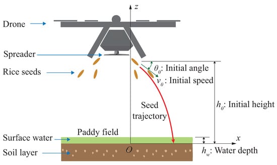
Figure 1 illustrates the trajectory of the rice seeds from the UAV when spreading to the impact of the soil bed, along with the global coordinate system that was used for dynamic analysis. The $xy$-plane represents the surface of the paddy field, with the z-direction perpendicular to the ground. Here, $v_0$ and ${\theta }_0$ denote the initial launching velocity and angle, respectively, placing the rice seed trajectory in the $zx$ plane.

Figure 2 illustrates the dynamic force equilibrium of a rice seed as it descends freely after being released from the UAV, including both a free-body diagram and a schematic diagram. The free-body diagram details the forces exerted on the seed, such as its weight, buoyancy, and drag force. In the schematic diagram, the inertial force components take into account not only the seed’s own inertia, but also the added mass effect. This effect arises as the seed moves through the fluid, displacing the surrounding medium and incorporating the inertia of the displaced fluid into the overall dynamics of the seed.

The equations of motion for the rice seed in the vertical and horizontal directions during falling are expressed as nonlinear ordinary differential equations (ODEs):

where z and x represent the position components of the rice seed in the global coordinate system. The double- and single-dot operators over the position components indicate the second and first derivatives with respect to time, respectively. Additionally, in Equations (1) and (2), m is the mass of the rice seed, $m_a$ is the added mass, $C_D$ is the drag coefficient, $\rho$ is the mass density of the surrounding fluid, $A=\pi R^2$ represents the projection area with R being the radius of the sphere, V is the volume of a rice seed, and $g=9.81\mathrm{m}/{\mathrm{s}}^2$ is the standard gravitational acceleration. The term involving the first-order derivative in Equations (1) and (2) corresponds to the drag force. The third term in Equation (1) represents the buoyant force, which can be neglected in the air domain. It is important to mention that the influences of the wind and paddy water flow on the falling rice seed were excluded from the motion equations to simplify the mathematical modeling and ensure numerical feasibility.

From a differential equation perspective, the non-linearity of Equations (1) and (2) arises not only because the drag force is proportional to the square of the velocity, but also because the drag coefficient is not constant and is instead a non-linear function of the particle Reynolds number, which is defined as follows:
where u represents the velocity of the fluid upstream relative to the sphere and $\mu$ denotes the dynamic viscosity of the fluid. The drag coefficient model used in this investigation, which was proposed by [23], was chosen because it is applicable to a wide range of particle Reynolds numbers that encompass both laminar and turbulent flow regimes, specifically $0.01<Re<$ 200,000:

The drag coefficient is determined by fixing a solid body in a wind tunnel or similar apparatus, then measuring the resistance force exerted by the fluid flow using a load cell. However, the rice direct seeding problem of the UAV involves a spherical body moving through a stagnant fluid. In this situation, the fluid is displaced by the moving spherical body, requiring the inclusion of an additional inertial force to accelerate the originally stagnant fluid, referred to as the added mass effect [24]. This phenomenon is referred to in this way because the coefficient of the second derivative term in the motion equations, i.e., Equations (1) and (2), is represented by adding $m_a$ to m. The added mass $m_a$ for a spherical body can be expressed as follows [25]:

The properties of air and paddy water used to establish equations of motion through Equations (1) and (2) for a rice seed that was assumed to be a sphere are summarized in Table 1. For the international standard atmosphere, the density and viscosity of the air is 1.225 $\mathrm{kg}/{\mathrm{m}}^3$ and $1.790\times {10}^{-5}\mathrm{Pa}·\mathrm{s}$, respectively [26]. In the paddy water domain, the material properties of a thin mud sample taken from a paddy field with a water content of 645.78% and a density of 1090 $\mathrm{kg}/{\mathrm{m}}^3$ were adopted from [27]. The paddy water exhibited Newtonian flow behavior, with a dynamic viscosity of $1.06\times {10}^{-2}\mathrm{Pa}·\mathrm{s}$ according to rheometer measurements.

To solve these differential equations, the initial conditions were given by ${\dot{z}}_0=-v_{0}sin({\theta }_0)$ and ${\dot{x}}_0=v_{0}cos({\theta }_0)$, with the initial positions being $z_0=h_0$ and $x_0=0$. The specific initial conditions for this numerical analysis were sourced from a review of the existing literature on UAV direct seeding experiments. Studies have concentrated on improving conditions for rice seed distribution [28,29,30]. In particular, the research conducted by Wu et al. in [28] offers essential information on the speed and orientation of the centrifugal spreading method. According to their findings, optimal conditions for maximum spreading uniformity are achieved with a UAV altitude of 2.1 m, a flight speed of 2 m/s, and a spreader baffle ring angle of 26°. The regression model derived from the data analysis indicates that, under these conditions, the relative velocity of rice seeds leaving the spreader is 0.63 m/s horizontally and 0.96 m/s vertically. Considering the UAV’s speed, the absolute horizontal velocity component ranges from 1.37 to 2.63 m/s. This corresponds to an initial velocity $v_0$ = 2.79 m/s and an angle ${\theta }_0$ = $18.9°$ for the maximum launch speed.

Regarding alternative seeding methodologies, the initial launch speeds for deploying the seed UAVs were derived from the research conducted by Lysych et al. [15] on the design of the seeding mechanism. For rice seeds released by the gravitational drop method, the vertical relative velocity with respect to the UAV is 0 m/s. When propelled using airflow, the relative vertical velocity is 18 m/s. In the case of pneumatic discharge, this relative speed can increase to 75 m/s. During pneumatic shooting, the seeds reach an average relative velocity of 225 m/s, with values ranging from 150 to 300 m/s, as reported in [31]. Pneumatic shooting, a term newly introduced in this study, describes the notably increased launch speed in relation to standard pneumatic discharge. A comprehensive summary of the absolute launch velocities and angles, incorporating both the relative discharge velocities and the horizontal speed of the UAV of 2 m/s for these five methods, is provided in Table 2.

Taking into account the variety in the launch velocity of rice seeds upon their release from the UAV, it was found that the Reynolds number of particles varied between $424\le Re\le$ 47,734 in air and $638\le Re\le$ 71,724 in water for the five sowing approaches, as detailed in Table 2. These Reynolds numbers fell within both the intermediate range ($1<Re<1000$) and the turbulent regime ($Re>1000$), where inertial forces took precedence over the laminar regime ($Re<1$) [21]. As a result, the drag force model described in Equation (4), which is applicable for $0.01<Re<$ 200,000, was clearly appropriate for the five seeding approaches analyzed in this research.

To improve the rice growth and yield, it is recommended to maintain the paddy water level at approximately 9 cm during sowing [32,33]. Therefore, for analyzing the flight dynamics of rice seeds sown from a UAV, the initial position conditions were set at a depth of 9 cm from the soil bed to the surface of the paddy water and a height of 2.1 m from the surface of the water to the UAV. This yields an initial height of $h_0$ = 2.19 m. Consequently, in the calculations of added mass, drag force, and buoyant force in Equations (1) and (2), the properties of the fluid were chosen based on the position of the rice seed, and the properties of the air or paddy water were selected accordingly. It should be noted that the added mass effect and buoyant force were not significant in the air region because the density of air is more than 800 times less than that of paddy water.

To solve the set of non-linear ODEs with the specified initial conditions and material properties, an in-house code was developed using the built-in ODE solver function ode23 in MATLAB version 2023a (developed by MathWorks, Inc. in Natick, MI, USA). The ode23 function implements the Bogacki–Shampine numerical integration scheme [34,35], which is based on an adaptive step size algorithm tthat is suitable for non-stiff problems like the free fall scenario analyzed in this study. Table 3 provides the calculated results for the terminal velocity and impact angle based on the initial conditions of the rice seed in the five different sowing mechanisms that are detailed in Table 2. These findings served as impact velocity conditions for performing the DEM simulations of the rice seed penetration that is described in Section 3.

Figure 3 exemplifies the calculated trajectory and velocity–time graphs of the rice seed that were obtained from the numerical integration of the non-linear ODE for the centrifugal spreading case among the five sowing methods. In Figure 3b, the path traced by rice seeds released from the UAV is shown, facilitating the estimation of the horizontal distance from the point of release to the point of landing in the paddy field. In this centrifugal spreading model, the rice seed covers an extra horizontal distance of 2.7 m in the UAV’s forward direction prior to reaching the field. Furthermore, when entering paddy water from the air, the velocity of the rice seed significantly decreases as a result of the higher viscosity of the water, as shown in Figure 3b.

In DEM analyses of the cohesive soils, the Hertz–Mindlin (HM) model combined with the Johnson–Kendall–Roberts (JKR) cohesion model has been extensively used [36,37,38,39,40]. The HM model is a contact model without cohesion that effectively and precisely characterizes the non-linear viscoelastic behavior of particle rheology through material constants and only a few parameters. The JKR model complements the cohesionless Hertz–Mindlin model by incorporating the cohesive forces between particles caused by moisture in fine powders or muddy soils. This paper provides a concise summary of the mathematical expressions of the contact models instead of presenting the entire formulation process for DEM equations of motion and contact models. This approach helps the reader understand the impact of the model parameters on particle behavior. In particular, this section presents excerpts from the previous paper of the author of [41], where the theory of contact models is introduced based on a review of the literature of references, such as [42,43,44,45] for the HM model and [46,47,48] for the JKR model.

Figure 4 illustrates a schematic of the contact condition between two spherical particles i and j, showing a normal overlap $\delta$ on the circular contact surface with a contact radius, which is denoted as a.

The Hertz–Mindlin model with JKR cohesion encompasses a Hertzian elastic force ${\mathbf{F}}_n^e$, a viscous force ${\mathbf{F}}_n^v$, and a JKR cohesive force ${\mathbf{F}}_n^c$ acting along the normal direction $\widehat{\mathbf{n}}$. In the tangential direction $\widehat{\mathbf{t}}$, as a cohesionless model, only the elastic force ${\mathbf{F}}_t^e$ and the viscous force ${\mathbf{F}}_t^v$ of the Mindlin elastic–viscous model were taken into account. In the equations provided in this paper, the boldface denotes vector quantities, while the italicized characters represent scalar quantities. A hat on a vector signifies a unit-directional vector with a magnitude of one. Each of the contact force components can be explicitly expressed in the following forms:

where $R_{\mathrm{eq}}$ is the equivalent particle radius, $E_{\mathrm{eq}}$ is the equivalent modulus of elasticity, ${\delta }_n$ is the normal contract overlap distance, e is the coefficient of restitution, $m_{\mathrm{eq}}$ is the equivalent particle mass, ${\mathbf{v}}_{\mathrm{rel}}$ is the relative velocity at the contact point, · is the vector inner product operator, $\gamma$ is the cohesive surface energy, a is the contact radius, $G_{\mathrm{eq}}$ is the equivalent shear elastic modulus, and ${\delta }_t$ is the accumulated tangential displacement during contact. The equivalent properties, which are denoted by the subscript eq, are expressed based on the individual properties of the particles i and j when they are in contact:

where $\nu$ is the Possion’s ratio.

In addition to the forces related to the translational motion expressed in Equations (6) through (10), the rolling friction ${\mathbf{M}}_r$ associated with rotational motion is modeled in the following simple form:

where ${\mu }_r$ is the coefficient of rolling friction, $\left|{\mathbf{F}}_n\right|$ the magnitude of resultant contact normal force, and $\mathit{\omega }$ is the particle relative angular velocity vector.

Simulating the bulk volume of systems with fine particles, such as soil or powder, becomes computationally infeasible with DEM if the particles are modeled at their actual size because of the sheer number of particles involved. To address this, DEM often uses an up-scaling approach, in which particle sizes are increased to reduce the number of particles and to improve computational efficiency to a feasible level [36]. This approach involves adjusting the contact model parameters to ensure that the behavior of the scaled-up particles closely mimics that of the original system of particles. A common theoretical approach to adjust the constants of the model, even when the size of the particle is modified, is the principle of similarity [49,50], which is achieved using the dimensionless parameters widely used in fluid dynamics analysis. However, the theoretical principle of similarity increases the structural geometry and computational domain in proportion to the particle size without reducing the number of particles to be computed. Consequently, this method does not offer any computational cost efficiency. Therefore, in DEM simulations of bulk soil, calibration techniques that effectively reduce computational burden are preferred over the principle of similarity. In bulk particle simulations based on the parameter calibration approach, the DEM particle size is initially determined considering both computational load and accuracy. The material properties such as density, Poisson’s ratio, and modulus of elasticity are typically kept at their original values. However, other parameters of the contact model, such as friction coefficients and cohesion model parameters, are calibrated against the experimental results of soil characterization tests, such as the slump test [36,38], the penetration test [51], and the measurement of the angle of repose [37].

In this research, rather than performing soil characterization tests and calibrating contact model parameters first hand, material properties and contact model parameters from previous publications were used for simulations. In particular, the properties of the rice seed material and the parameters of the contact model were obtained from [19], which also provided shape information. Figure 5 illustrates the CAD (computer-aided design) geometry along with its multi-sphere model for DEM analysis. Initially, rice grain was represented in CAD as a spheroid, which is characterized by a semi-major axis of 4.5 mm and a semi-minor axis of 1.05 mm. Subsequently, this spheroid was discretized into a configuration of seven spherical particles, as shown in Figure 5, with the x-directional position and radius of each sphere detailed in Table 4. The variability in the size of the rice seeds affected their aerodynamic characteristics and ability to penetrate the soil, as these depend on variations in mass, drag force, and impact resistance. However, in this study, the velocities at which the seeds were discharged from the UAVs surpassed the expected variability range of seed sizes. Given this study’s relatively low sensitivity to seed size variation, the statistical distribution of rice seed sizes was omitted from the simulations.

It is important to note that if the soil particles are larger than the rice seed, the rice seed could easily penetrate the interstitial spaces between the soil particles, which would reduce the reliability of the penetration simulation results. Consequently, in this DEM analysis, a soil particle size of 0.5 mm was chosen, which is less than half of the semi-minor axis of 1.05 mm of the spheroidal rice model, as shown in Figure 5. The material constants and contact model parameters for the paddy soil were determined by referring to [36,37,38,39,40,52,53,54,55]. Specifically, the parameters required for DEM simulations were extracted from [55], except for the surface energy for the JKR cohesion. The surface energy of the soil particles was taken from [37], which describes DEM simulations on soil particles to assess the angle of repose through a steepest ascent test. Since, to the best of the author’s knowledge, no existing publications have provided DEM calibration constants for the contact interaction between rice grain and soil, this study assumed that these constants were the mean values of the two materials. In DEM simulations, the computational domain of the paddy field cannot be infinitely expanded. This requires selecting a limited computational region and specifying boundary walls to contain the particles. The contact parameters between these boundary walls and the soil particles were set to be the same as those for soil–soil interactions. The characteristics of the materials and the contact model parameters relevant to DEM calculations for rice and soil are detailed in Table 5 and Table 6, respectively.