Enhanced Neonatal Brain Tissue Analysis via Minimum Spanning Tree Segmentation and the Brier Score Coupled Classifier

1. Introduction

Neonatal brain MRI segmentation is of paramount importance for assessing and managing brain damage and disorders arising from premature births [1]. Preterm birth increases the risk of brain injury, often leading to further neurodevelopmental impairments [2]. The precise segmentation of brain MR images, distinguishing between various tissue categories, is a critical initial step in detecting disease-specific morphological variations [3]. These tissue categories, including gray matter (GM), white matter (WM), and cerebrospinal fluid (CSF), as well as other functional structures, play a pivotal role in neuroimaging studies [4].

Automatically segmenting an image into its diverse components remains a significant challenge [5], and despite two decades of development in segmentation techniques, many approaches still require user intervention [6]. Enhancing reproducibility through automation is a critical goal [7]. Probabilistic atlases have been widely used, but their effectiveness relies on stable magnetic resonance sequences and multispectral information for training and tissue specification [8,9]. Perinatal brain imaging, marked by rapid morphological changes and increased motion artefacts, poses unique challenges that make traditional voxel-based intensity classification approaches impractical [10,11].

The existing literature has introduced newborn brain templates and probability maps for CSF, WM, and GM [12], aiding registration and serving as prior information for newborn brain segmentation. The rapid growth of the fetal brain during early pregnancy, especially in premature infants, underscores the heightened risk of cognitive and behavioral impairments [13]. Neonatal brain segmentation often relies on atlas-based methods, posing challenges in dealing with non-homogeneous intensity distributions, background noise, complex shapes, uncertain boundaries, and minimal intensity differences [14,15].

The maturation of white matter tissue into non-myelinated and myelinated categories introduces further complexity, with non-myelinated WM exhibiting distinct intensity profiles in neonates compared to adults [16,17]. Traditionally, tissue intensities’ probabilities have been modeled by employing finite mixture (FM) and finite Gaussian mixture (FGM) methods [18].

MRI studies on neonatal brain development have been limited, often involving scans of sedated neonates and young children [19]. The challenge of enhancing classifier accuracy has been addressed through feature selection, emphasizing the need for fewer yet more discriminative features [20].

1.1. Motivation

The motivation for this research was from the urgent need to enhance neonatal brain structure analysis using MRI. The existing methods face challenges such as low-intensity contrast and the dynamic nature of brain tissue development, leading to suboptimal segmentation and classification results. This research aimed to contribute a novel approach that would address these challenges, providing a more accurate and efficient solution for neonatal brain image analysis. The goal was to advance the field by introducing innovative techniques and methodologies, ultimately improving our understanding of neonatal brain development and contributing to more effective diagnosis and monitoring of neurodevelopmental disorders.

1.2. Related Work

In recent research related to the segmentation and classification of neonatal brain structures, several notable studies have been discussed:

Ioannis S. Gousias et al. [21] created methods for manually segmenting cerebral MR images of newborns into 50 distinct regions. The study involved 15 preterm infants and five term-born infants, and the authors carried out estimation of total and regional brain volumes, pre-processing, co-registration, and segmentation using a region-of-interest approach. Feng Shi et al. [22] developed a Learning Procedure for Brain Extraction and Labelling (LABEL) for newborn MR brain images. The method involves a meta-algorithm for multiple brain extractions with a Brain Surface Extractor and Extraction Tool. The authors developed a fusion method based on level sets. The system achieved more accurate brain extraction on 246 subjects, outperforming other methods. Dwarikanath Mahapatra [23] developed a graph-cut method for neonatal brain skull stripping from MRI scans using prior shape information. This method accurately identified brain and non-brain tissues, with pixel probabilities and a smoothness term. The experimental results showed its superiority over traditional segmentation methods. Cardoso et al. [24] developed AdaPT, an adaptive, preterm, multi-modal, maximum a posteriori expectation-maximization segmentation algorithm. It improved image segmentation, particularly for the cerebellum, pathological cortical gray matter, and ventricular volume, and demonstrated significant improvements over the widely used algorithm. Antonios Makropoulos et al. [25] presented a precise segmentation scheme for neonatal brain MRIs, dividing them into 50 brain regions, beginning with preterm images and ending at those for neonates of a term-equivalent age. This segmentation algorithm incorporated structural hierarchy and anatomical constraints to model brain intensities across the entire brain. A comparative analysis with conventional atlas-based segmentation methods revealed an improved label overlap with manual segmentation. The proposed methodology exhibited high precision and robustness throughout a broad span of gestational ages, from 24 weeks’ GA to a term-equivalent age. In Richter and Fetit’s research, they developed a DL-based channel for newborn brain MRI segmentation, demonstrating the potential of transfer learning to overcome limited annotated data. While successful in many aspects, challenges were identified in segmenting specific tissue classes such as the cerebellum, suggesting a need for further investigation into the distinct biological variations between normal and premature infants to improve segmentation accuracy [26]. Boswinkel et al.’s [27] study on brain lesions in moderate–late preterm infants found that mild lesions, such as small hemorrhages and white matter injury, were more common in these infants. The study used MRI and cranial ultrasound to assess brain lesions, but limitations were not including infants with a gestational age of 36 weeks and missing data for some infants. Further research is recommended to assess the clinical relevance and neurodevelopmental outcomes. Another study [28] explored motion artefacts in neonatal brain MRI scans, highlighting the need for tailored motion correction techniques. It suggested intensity-based interpolation as a potential solution, but acknowledged limitations such as a potential ineffectiveness in severe cases and varying impacts on segmentation results. Further research is needed for a compatibility of interpolation techniques. The authors of [29] proposed a 3D-cycle GAN-Seg architecture for generating synthetic images of the isointense phase, where a consistency in tissue segmentation between images of 6-month-old and 24-month-old subjects was ensured. They propose a feature matching loss to improve the synthetic image quality, and the addressed brain shape deformation between time points. Owing to the brain’s rapid expansion over time, the distortion of the brain’s geometry among two points in time will be an intriguing issue to study. Makropoulos et al. [30] examined and classified approaches used for the prenatal brain based on a target population, certain segmentation structures, and a specific methodology. This analysis concluded with a discussion of the perinatal domain’s weaknesses and the future prospects. Chen et al. [31] proposed a newborn brain extraction scheme built on autonomous deep learning, which works well on both high- and low-resolution MRIs. This research focused only on brain portion extraction from MR images. Beare et al. [32] introduced a newborn tissue segmentation technique called MANTiS segmentation and classification for brain damage and growth linked to premature delivery. The performance of MANTiS was evaluated on two separate databases, showing promising results in segmenting neonatal brain tissues. The authors outlined the segmentation of various brain tissues in preterm infants using MANTiS, highlighting its potential for neuroimaging research. But the age group considered was limited. Ding et al. [33] reported on the use of deep CNN to segment newborn brain images. Their study compared two neural network architectures for segmenting neonatal brain tissue types and evaluated their performance. The study aimed to exhibit the usability and reproducibility of these networks for newborn brain segmentation. However, the limitations of the study included a small sample size of data with labels and a need for continual retraining of the networks for improved performance. The work emphasized that deep neural networks may offer an alternative and have the scope to be used in neonatal brain tissue analysis. Vaz et al. [34] provided different approaches for extracting brain images from MRI scans of preterm infants. Their study evaluates the accuracy of automated methods compared to manual segmentation and assessed the impacts of different methods on intra-cranial volume measurements. The study also discussed the computation time for each technique and the reliability of manual segmentation. Limitations of the study included its small dataset and the potential impact of brain lesions on the segmentation accuracy. The authors emphasized the importance of accurate brain extraction for medical imaging and provided insights into the performance of specific automated methods.

These studies have collectively contributed to advancing the field of neonatal brain image segmentation and classification, addressing critical challenges in pediatric neuroimaging. Table 1 provide a comparison table summarizing the key aspects of the recent studies on the segmentation and classification of neonatal brain structures.

1.3. Research Gaps

Previous studies in neonatal brain tissue segmentation have made valuable contributions, yet certain research gaps persist. One notable gap is the limited exploration of efficient pre-processing techniques to mitigate motion artefacts in neonatal brain MRI. Additionally, the challenge of distinguishing unmyelinated and myelinated white matter in the segmentation process remains underexplored, with existing methodologies relying on conventional approaches. Furthermore, the need for a fully automatic system capable of classifying a comprehensive range of neonatal brain tissues with minimal human involvement has not been adequately addressed.

This work directly addresses the identified gaps in the related literature. We propose innovative pre-processing techniques to effectively correct motion artefacts in neonatal brain MRI, contributing to an improved data quality for segmentation. Our methodology also tackles the nuanced task of distinguishing white matter that is unmyelinated or myelinated, offering a more refined approach compared to conventional methods. Additionally, our research introduces a robust, fully automatic system that maximizes the classification of neonatal brain tissues, filling a critical void in current practices.

Segmenting neonatal brain tissues presents unique challenges due to the rapid growth processes, motion artefacts, and need for comprehensive classification. Existing methodologies often lack the precision and automation required for a thorough analysis. Our research aimed to bridge these critical gaps by developing an innovative segmentation method using the minimum spanning tree (MST) with the Manhattan distance, addressing challenges related to growth and motion artefacts. Additionally, we integrated advanced classification techniques, coupling the Brier score with the shrunken centroid classifier, to enhance precision and reduce manual interventions. Our objectives included comprehensive tissue identification, minimization of human intervention through a fully automatic system, comparative analysis against existing methods, efficient pre-processing for motion artefact correction, and evaluation of the clinical relevance in neonatal healthcare. In setting these objectives, we aimed to advance the state of the art in neonatal brain tissue analysis, contributing to improved healthcare outcomes and a deeper understanding of neurodevelopmental disorders.

1.4. Contributions

This research paper makes several significant contributions to neonatal brain tissue investigation and classification:

(a): Enhanced Neonatal Brain Tissue Segmentation: Our work presents an innovative approach for segmenting neonatal brain tissues, overcoming the challenges posed by rapid growth processes and motion artefacts commonly encountered in neonatal brain MRI. We employ cutting-edge techniques, such as minimum spanning tree (MST) segmentation with the Manhattan distance, to increase the robustness and accuracy of segmentation.
(b): Advanced Classification Methodology: We presented a novel classification scheme by coupling the Brier score with the shrunken centroid classifier. This hybrid approach enhances the accuracy of tissue classification, leading to more precise and reliable results. It also reduces the dependency on manual interventions and establishes a foundation for fully automatic segmentation and classification.
(c): Efficient Tissue Identification: Our methodology addresses the identification of various neonatal brain tissues, including myelinated and unmyelinated white matter, while mitigating the challenges posed by partial volume effects. By enhancing tissue discrimination, we contribute to a more comprehensive understanding of neonatal brain structures.
(d): Minimized Human Intervention: We emphasize the importance of reducing human intervention in the segmentation and classification process. Our system aims to be a fully automatic solution, minimizing the need for manual adjustments and interventions, thus streamlining the workflow and enhancing efficiency.
(e): Increased Tissue Coverage: In contrast to previous works that segmented a limited number of neonatal brain tissues, our approach endeavors to classify the maximum number of brain tissues with significantly reduced human effort. This expansion in tissue coverage contributes to a more comprehensive analysis of neonatal brain structures.

In summary, our paper presents an integrated framework that not only addresses the challenges of neonatal brain tissue segmentation and classification but also contributes to the goal of creating a robust, automated system for characterizing neonatal brain structures. These contributions collectively to advancing the state of the art in neonatal brain image analysis, with potential suggestions offered for an improved diagnosis and treatment of neurological disorders in neonates.

The rest of this article is organized as follows: Section 2 discusses the proposed approach. The implementation part of our work is then discussed in detail in Section 3. Section 4 describes the dataset used for experimentation briefly. The quantitative and qualitative analysis outcomes based on the obtained results are then given in Section 5. Finally, this article is concluded in Section 6.

3. Implementation and Analysis

The proposed methodology can be effectively implemented using the MATLAB 2013b platform. To evaluate its performance and compare it with conventional methods, we conducted comprehensive experiments and analyzed the results.

As depicted in Figure 2, the inputted neonatal image from the database undergoes pre-processing steps such as Wiener filtering for noise removal, realignment for motion correction, and a combination of N3 and information minimization for intensity inhomogeneity correction. Subsequently, texturing features are taken from the pre-processed image through DTCWT, and then the most relevant features are selected using the Isomap technique. Based on these selected features, the image undergoes segmentation via MST segmentation modified with the Manhattan distance. Tissues are then classified from the segmented image. Each of these processes is detailed in the subsequent sections.

3.1. Model and Problem Formulation

The brain of a neonate differs significantly from that of an adult. While the adult brain is fully developed, the neonatal brain is still in the developmental stage. Additionally, the neonate brain is much smaller in size, and the movement of fluids within the brain during a scan makes it challenging to distinguish between different tissues. Here, an advanced method for processing newborn brain images is necessary to overcome the complications. In our research, we used a hybrid technique by integrating minimum spanning tree segmentation and the Brier score coupled with the shrunken centroid classifier for classifying newborn brain tissues. The database D contains N number of images and can be represented mathematically as

$D = {I_{i}}_{i = 1}^{N}$

(1)

From this database, the image I is taken, and each of the processes in neonatal brain image segmentation and classification are explained below.

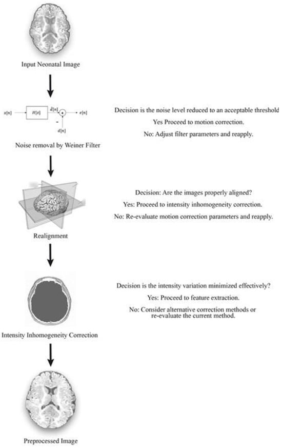
3.2. Pre-Processing (Stage-1)

Pre-processing is the first stage of preliminary processing. It includes cleaning, sampling, normalization, and transformation of the image. The crucial role of pre-processing is to transform the neonatal brain image into a format that will be more easily and effectively processed in subsequent steps. The three pre-processing steps used in our research work were Wiener filtering, realignment, and intensity inhomogeneity correction. The filtering process was used to remove both neonatal brain image noise as well as image blurring. Motion correction was performed in the realignment process and, finally, intensity correction was carried out via the inhomogeneity correction method.

3.2.1. Wiener Filtering

A Wiener filter is a linear time invariant (LTI) filtering method using a statistical estimate of an unknown image [35]. By comparing the input neonatal brain image corrupted by additive noise (desired) with a standard neonatal brain image (estimated), it minimizes the mean square error (MSE) among intended and predicted processes at random to remove both image noise as well as image blurring. Every pixel is an advanced representation of the neonatal brain image, which serves to convey to the force of a solitary stationary point before the image; if the shade pace is too moderate and the neonatal brain image is in movement, a given pixel will reflect a fusion of intensities from focuses along the line of the movement. The Wiener filter is a frequency domain filter and it is mostly used in frequency domain analysis. Initially, the power spectrum of the image was estimated or the mean of the power spectrum of a large set of images was estimated, which was used as the power spectral input of the Wiener filter and measured the average of the squares of the errors or derivations between them, that is, the mean squared error (MSE), which can be calculated by using the formula,

$M S E = \frac{1}{N} \sum_{i = 1}^{n} {({\overset{ˇ}{x}}_{i} - x_{t})}^{2}$

(2)

where N = total number of images, ${\overset{ˇ}{x}}_{i}$ = mean of the power spectrum of images N, and $x_{t}$ = power spectrum of images I_i. By reducing the mean square error of the neonatal brain images, the input images are converged to perfection and hence the noise is reduced. After removing noise from the images, the motion artefacts may be minimized with the help of realignment, and this is explained in the following section.

3.2.2. Realignment

The filtered neonatal brain image obtained from the former step is then realigned to reduce motion artefacts. As neonates will not be stationary during the scanning process, because of their mental unawareness, the image undergoes important motion artefact removal. Generally, the atlas method is used in newborn brain scanning for image registration and labeling processes. But, in this research, we implemented a realignment method where instead of an atlas or a reference image, the input neonatal brain image itself was compared with another input neonatal brain image taken at a different time interval (T1 and T2 images). Image matriculation involves spatially adjusting the objective image(s) to the enlisted reference images [36].

First, a reference neonatal brain image is chosen; here, input neonatal brain images taken in different time periods are used, typically to realign each succeeding scan. These processes, such as rotation and translation, are executed through matrices. The difference function for transformation of an image can generally be expressed in the form,

$d_{i} (p) = f (s (x_{i}, p_{s})) - t (x_{i}, p_{t})$

(3)

where $f (s (x_{i}, p_{s}))$ is a vector function that describes changes in space depending on parameters, $p_{s}$ = (Pitch, Roll, Yaw), and $t (x_{i}, p_{t})$ is the scalar function that describes the intensity transformation depending on parameter $p_{s}$ = (Pitch, Roll, Yaw).

The intensity of every pixel in the changed image can essentially be resolved from the intensities in the first image. Keeping in the mind the end goal to realign the image through subvoxel precision, spatial changes will include portions of a voxel, resulting in the establishment of a precise correlation among reference and target images. After realignment, the intensity variance in pixels is optimized. Once the correction of motion in the neonatal brain image is completed, the presence of intensity inhomogeneities is removed through the combination of the N3 method and information minimization techniques, as explained in the following section.

3.2.3. Intensity Inhomogeneity Correction

The intensity inhomogeneity is the variation in intensity at different points of the image, such as slowly varying shading artefacts. It is also known as the bias field in medical images. Intensity inhomogeneity in MRI neonatal brain images can significantly decrease the precision of division and transformation of images. In spite of advances in terms of revising spatial power inhomogeneity in present-day scanner programming, the appearance of multi-channel staged cluster curls and 7T+ scanners have expanded (once more) the significance of this issue for post-check handling. An issue for division apparatuses that depend on the developed methodologies is that a white matter voxel at one point in the image may have the same intensity as a gray matter voxel in different areas of the image. Background cleaning, white matter identification, and bias field valuation inside the white matter voxel can be conducted via intensity inhomogeneity correction. In our methodology, bias field correction [37] is carried out through a combination of the non-parametric, non-uniform intensity normalization (N3) method and the information minimization method. The N3 method is used to estimate the intensity inhomogeneity field (IIF), and information minimization minimizes the IIF.

3.3. Non-Parametric, Non-Uniform Intensity Normalization (N3)

This method does not rely on the pulse sequence, and the estimation of dissimilar intensities is shaped by this technique. Bias correction is applied to images of intensities in order to minimize entropy. One advantage of this approach is that it can be used early in an automated data processing procedure, before a tissue model is accessible. For the purpose of calculating intensity variation, an iterative method is utilized to estimate the multiplicative bias field as well as the true tissue intensities’ distribution.

The first step in the N3 algorithm [38] is obtaining the probability densities V, F, and U. V is simply the histogram of log intensity for neonatal brain MR image

I_{i},

which is the only measurable distribution; F and U must be estimated. Bias field F is well estimated by a unimodal Gaussian distribution. To approximate F, a Gaussian kernel with a full width at half maximum (FWHM) of 0.1 was employed. U can be estimated by the way of the following deconvolution filter:

$\tilde{G} = \frac{\tilde{F} *}{{\tilde{| F |}}^{2} + Z^{2}}$

(4)

where $\tilde{F}$ = the Fourier transform of $F$ , $Z$ = a constant term to limit the magnitude of $\tilde{G},$ and U = a distribution function.

The N3 calculation for non-consistency revision makes no presumptions about the intensity of conveyance of fundamental tissue. Instead, U is evaluated non-parametrically from the data by deblurring the deliberate sign intensity V. An assessment of the predisposition field is then derived from the proposed U and y used to adjust the first image. This corrected neonatal brain image is then inputted into the calculation for further redressing. When F or U quits changing with extra cycles, and no more change can be accomplished, the calculation has achieved its objective. After that, information minimization is performed to minimize the impact of intensity inhomogeneity, and this is explained in the following section.

3.3.1. Information Minimization

The information minimization technique is used to minimize or reduce the intensity variation. The elimination of a very higher intensity or very low intensity is based on the average method. In an MR neonatal brain image, intensity varies with respect to location, that is, some regions have a high intensity when compared with neighboring regions, and some regions may have a very low intensity when compared with neighboring regions. This variation in intensity has to be minimized. That minimization is performed by a linear model of image degradation. Initially, we depict the modeling phase, whereby the model’s parametric correction is defined. Second, we describe how to determine the best correction model and calculate the corresponding updated image. An information minimization technique is commonly used in all fields. In this technique, a lower limit and higher limit are set, where the selection of limits is based on the extremity of the intensity. The intensities that are found outside of the limits are minimized to the average value of the limits.

Modelling of Information Minimization Method

The linear model of image degradation consists of a multiplicative

m (x)

and an additive

a (x)

intensity degradation component.

$v (x) = u (x) m (x) + a (x)$

(6)

When at location

x_{i}

v (x)

is the measured signal,

u (x)

is the true signal emanating via tissue,

m (x)

is the unidentified smoothly varying bias field, and

a (x)

is the white Gaussian noise, assumed to be independent of

(x)

. The difficulty in making up for intensity non-uniformity arises in approximating

m (x)

, which can be based on the deterioration model’s inverse, provided by Equation (7):

$\tilde{u} (x) = v (x) {\tilde{m}}^{- 1} (x) + {\tilde{a}}^{- 1} (x)$

(7)

where ${\tilde{m}}^{- 1} (x) = \frac{1}{m (x)}$ and ${\tilde{a}}^{- 1} (x) = - \frac{a (x)}{m (x)}$ .

After calculating the inverse degradation model, the intensities must then be corrected, and this is explained in the following section.

3.3.2. Correction of Brain Image

True image

u (x)

covers exclusive information related to the imaged object, which is first multiplied by

m (x),

and next, the noise

a (x)

is added to it. Transformation of the acquired neonatal brain image

v (x)

into the optimally corrected image

u_{2} (x)

proceeds as follows:

$u_{2} (x) = F [u (x) m (x)] + a (x)$

(8)

In this equation, “F” represents a noise-reducing filter applied to the product of $u (x)$ and $m (x)$ . Hence, in the pre-processing section, we reduced the noise level, blurring, motion artefacts, and the intensity inhomogeneity correction, which made the image’s feature extraction more precise. The feature extraction process using DTCWT and the Isomap technique is explained in the following section.

3.4. Feature Extraction (Stage-1)

This is a dimension reduction process that effectively conveys a captivating portion of an image as a small feature, where extracted features are anticipated to contain appropriate information from the input data. Feature extraction can be explained, in general, as narrowing down data from a large number of resources in order to perform an analysis. When analyzing complex datasets, a significant challenge is managing the numerous variables involved. Handling a large number of variables often demands substantial memory and computational resources. Additionally, it can lead to overfitting in classification algorithms. Feature extraction refers to techniques used to combine variables to address these challenges while still accurately representing the data. In image processing, it involves using algorithms to identify and isolate specific parts or shapes of interest. There are many techniques that are used in image processing to extract features. Our methodology utilizes the Dual Tree Complex Wavelet Transform [39], where both feature selection and feature extraction are carried out in a single step.

Neonatal brain MR images offer valuable insights into the structure and development of the infant brain. To extract meaningful information from these images, various features are computed. Textural features capture the spatial arrangement of pixel intensities, providing information about the patterns and structures within the tissue. Intensity features, derived from pixel values, reveal the brightness and color distribution. Shape features describe the geometric properties of segmented regions, such as the area, perimeter, and compactness. Frequency domain features, extracted using the Dual Tree Complex Wavelet Transform (DTCWT), provide insights into the structural characteristics of the images. Finally, statistical features, such as skewness and kurtosis, summarize the distribution of intensities within a region. By combining these features, researchers can gain a deeper understanding of brain development and identify potential abnormalities.

3.5. Dual Tree Complex Wavelet Transform

The Dual Tree Complex Wavelet Transform (DTCWT) [39] is an enhancement of the Complex Wavelet Transform (CWT) and Discrete Wavelet Transform (DWT). It extracts features from neonatal brain images by decomposing them into real (tree “a”) and imaginary (tree “b”) parts using specially designed low-pass filters that differ by half a sample period. These filters are reversed between the two trees to generate real and imaginary coefficients.

The image is divided into up to six levels, producing multi-scale, multi-directional sub-bands that enhance high-frequency details and reduce noise. The synthesized output is further denoised using wavelet transformation. DTCWT provides improved directional selectivity and reduced shift variance compared to standard DWT, making it effective for neonatal brain imaging. It also exhibits less redundancy than the un-decimated (stationary) DWT, making it more efficient. The output from DTCWT can be represented by the following equation:

$φ (t) = φ_{R} (t) + j φ_{J} (t)$

(9)

where $φ_{R} (t) and φ_{J} (t)$ are wavelets generated by the two DWTs. Phase and amplitude information is computed using the real and imaginary coefficients. The Dual Tree Complex Wavelet Transform (DTCWT) divides sub-bands into positive and negative orientations using two distinct discrete wavelet transform decompositions. The real and imaginary components are computed through real tree filters (h0 and h1) and fictitious tree filters (g0 and g1), respectively. As shown in Figure 3, DTCWT offers superior directional selectivity and reduced shift variance compared to previous methods. Unlike the critically sampled DWT, which has a 2D redundancy factor for multi-dimensional data, DTCWT provides an improved efficiency with less shift variance and lower redundancy compared to the un-decimated DWT.

The DTCWT is a feature extraction technique that decomposes neonatal brain images into real and imaginary components as depicted in Algorithm 1. It offers improved shift invariance and directional selectivity compared to traditional wavelet transforms, leading to more robust feature extraction and better segmentation outcomes.

Algorithm 1. for DTCWT

1 Set i = 1 and yield the DTCWT of the input image.
2 Set zero to all wavelet coefficients with the level lesser than a threshold

θ_{i}

.
3 Proceeds DTCWT-1 and calculate the inaccuracy owing to loss of lesser coefficients.
4 Take DTCWT of the error neonatal brain image and adjust the non-zero wavelet coefficients from step 2 to lessen the error.
5 Increase i, lesson

θ_{i}

the slightly (to comprise a few more non zero coefficient) and recap steps 2 to 4.
6 When there are enough non zero coefficient to provide the essential rate-distortion trade off, Keep

θ_{i}

constant and repeat a few extra times until converged.

Features can vary in relevance: they can be most relevant (containing unique information), relevant (containing some information also found in other features), or irrelevant. Generating a diverse set of features is crucial. Therefore, feature selection is used to select the most relevant features, and here, the Isomap technique is applied.

3.6. Isomap Technique

The Isomap technique is used to reduce the number of variables under a certain condition. As the result of DTCWT, the number of extracted features was increased. If all these features were implemented in segmentation, it would be complex. So, the accuracy of neonatal brain segmentation is reduced to avoid this, where only some vital features are selected for the next process of segmentation. The loss of useful data during data selection is thereby minimized. Isomap is a nonlinear dimensionality reduction method that belongs to the family of isometric mapping strategies, akin to multidimensional scaling (MDS). It constructs low-dimensional embedding by preserving geodesic distances derived from a weighted graph. Specifically, Isomap utilizes the geodesic distance defined by the shortest path along the graph edges, to capture complex structures in the resulting embedding. The top n eigenvectors of the geodesic distance matrix represent the directions in the new n-dimensional Euclidean space [40].

In the steps involved in the Isomap technique, the neighbor of every point is determined within a fixed radius. The nearest neighbor is taken as k and then we construct a graph by connecting each point, whereas the Euclidean distance is determined by the edge length. By using Dijkstra’s algorithm, Floyd–Warshall algorithms find the shortest distance between two nodes.

The initial step identifies neighboring points on the manifold M, based on distances $d_{X} (i, j)$ between pairs of points i and j in the input space X. Subsequently, each point is connected to its K nearest neighbors. These neighborhood relationships are depicted as edges in a weighted graph G over the data points, where the edges have weights $d_{X} (i, j)$ based on the distances between neighboring points i and j in the input space X.

The second phase involves Isomap estimating geodesic distances

d_{M} (i, j)

between all pairs of points on the manifold M by determining their shortest path distance

d_{G} (i, j)

within the graph. Subsequently, metric multidimensional scaling (MDS) is applied to compute the distance matrix of the graph. Coordinate vectors

v_{i}

for points in Y are then chosen to minimize the following optimization function:

$E = {‖ τ (D_{G}) τ (D_{y}) ‖}_{z^{2}}$

(10)

where $D_{y}$ denotes the matrix of Euclidian distances, the τ operator coverts distances to inner products, and $L^{2} = \sqrt{\sum_{⋁} A_{⋁}^{2}}$ . Then, we eliminate the lower dimensional features using the multidimensional scaling method. The obtained feature values are then mapped to the pixel locations present in the image. After the feature extraction process, the image undergoes segmentation.

3.7. Minimum Spanning Tree with Manhattan-Distance-Based Segmentation

Segmentation of newborn brain images refers to the process of dividing or partitioning a digital image into distinct parts or sets of pixels. The main goal of segmentation is that changing the color, intensity, or texture of a desire region so it makes more sense and is simpler to analyze. This segmentation is the process of assigning a label to each pixel in an image so that pixels sharing the same label exhibit specific attributes. Segmentation covers the whole image, where neighborhood regions exhibit substantial variations in similar characteristics. This approach is often employed to detect objects or relevant features within digital images. Common segmentation techniques in image processing include region-based, threshold-based, and edge-based segmentation. But perfect newborn brain image segmentation can be achieved by using the minimum spanning tree with the Manhattan distance. MST segmentation is modified here with the Manhattan distance, which is a dimension-independent distance.

The minimum spanning tree is a graphical partitioning method [41]. Graph apportioning strategies serve as valuable tools for segmenting images of the newborn brain. These strategies model the influence of pixel neighborhoods on a designated group of pixels, assuming homogeneity across images. In these methods, the image is represented as a weighted, undirected graph where individual pixels or groups of pixels serve as nodes, and edge weights indicate dissimilarities between neighboring pixels. The newborn brain image is subsequently segmented based on criteria tailored to cluster modeling. Each partition of nodes or pixels produced by these algorithms is interpreted as an object segment within the image. Formally, for a graph

G = (V, E)

, the spanning tree is

E_0 \subseteq E

, such that

$\exists u \in V : (u, v) \in E_0 \lor (v, u) \in E_0 \forall v \in V$

(11)

where $V$ represents a set of vertices in the graph, and $E_0$ represents a subset of the edges of the graph.

The subset of edges spans all vertices. The distance between two points is classically calculated by means of the Pythagorean Theorem. But one of the effective methods of finding the shortest distance between two points is the Manhattan distance. This is the distance between two points measured along perpendicular axes. In our research, the Manhattan distance was used to find the similar pixels or similar regions in the segmentation process. The map assigns a distance value to each pixel in the image based on its proximity to the nearest obstacle, where pi is the closest pixel causing an obstacle.

The minimum spanning tree technique divides the neonatal brain image up in the form of a grid, and each pixel in the grid is considered the vertex in a graph. A single graph can have multiple spanning trees, each connecting all vertices with the minimum total edge weight. The acquired information from each pixel is stored in the data structure. Kruskal’s MST algorithm is used in the segmentation process, and the edges between the neighborhood pixels are formed then by employing the Euclidean distance, which refers to the distance between two points in Euclidean space. Edge weightage is the measured pixel similarity, which is judged by a heuristic method that compares the weight to a per-segment threshold.

In a grid, the distance between two points is calculated based solely on horizontal or vertical paths, with no diagonal movement considered. The Manhattan distance, a dimension-agnostic measure, is obtained by summing the horizontal and vertical components, also known as the L-1 distance. For two points,

u = (x_{1}, y_{1})

and

v = (x_{2}, y_{2})

, the Manhattan distance between u and v is defined as

$M H = | x_{1} - x_{2} | + | y_{1} - y_{2} |$

(12)

where $x_{1}, y_{1}, x_{2}, and y_{2}$ are points on a plane.

The Manhattan distance between u and v can be generalized as

$M H = \sum_{i = 1}^{n} | x_{i} - y_{i} |$

(13)

Minimum spanning tree (MST) segmentation using the Manhattan distance is a robust method for partitioning neonatal brain images into meaningful regions. This approach enhances image clarity for diagnostic and research purposes in neurodevelopmental disorders. The Manhattan distance, known for its dimension-independent effectiveness, identifies similar pixels and regions, improving segmentation accuracy. The MST algorithm connects neighboring pixels based on Euclidean distances, with edge weightage determined heuristically. The Manhattan distance, calculated as the sum of horizontal and vertical components, serves as a reliable similarity measure. In summary, the MST with Manhattan-distance-based segmentation is a valuable tool for neonatal brain image analysis, offering enhanced precision and applications in neuroimaging research concerning the gyrus, myelinated white matter, unmyelinated white matter, medial part, lateral part, occipital lobe, cerebrospinal fluid, and temporal gyrus. The overall process involved in the segmentation of newborn brain images can be summarized in the following manner.

3.8. Grid Formation

Divide the pre-processed image U(x) into a grid format where each of the pixels $u_{i} (x, y)$ in the image is represented as a vertex in the graph. In the process of grid formation, the information about the pixels is stored in the data structure (DS).

Among every pixel in the graph, a link between the vertices will be form based on the degree of neighborhood between them, and that is measured through the Euclidean distance calculation, as given in the following Equation (14). Consider that the two vertices in grid formation are

u_{i} (x, y)

and

u_{j} (x, y)

, based on these, the degree of neighbourhood is measured,

$d (n) = \sqrt{{(u_{i} (x, y) - u_{j} (x, y))}^{2}}$

(14)

Here, the degree of neighborhood is measured in terms of the feature values obtained in the feature extraction phase. After finding the neighborhood between the nodes, they are sorted, and this is explained in next section.

3.9. Edge Sorting

Edge sorting is a crucial step in image segmentation that involves organizing edges based on their similarity. It facilitates efficient region merging, ensuring accurate and meaningful segmentation.

Procedure:

Weight Calculation: Calculate the weight of each edge using the Manhattan distance.
Sorting Edges: Sort the edges in ascending order based on their weights.
Merging Criteria: Merge regions based on predefined criteria, starting with the lowest-weight edges.
Dynamic Adjustment: Adjust merging criteria based on the image context or analysis requirements.

Edge sorting enhances segmentation quality by ensuring that similar regions are merged first, leading to more coherent and anatomically accurate segmentations. This is particularly important in medical imaging.

In this process, an edge emerges among each pair of nodes; as a result, a set of edges $e (u_{i}, u_{j})$ will be formed in the images, and the edges are sorted in ascending order. After that, the merging criterion is checked, and the regions are merged as given in the following section.

3.10. Pixel Merging

After sorting the edges based on their weights, the region similarity between every edge is calculated through the Manhattan distance, and hence Equation (14) is modified as Equation (15):

$M H (u_{i}, u_{j}) = \sum_{i, j} | u_{i} - u_{j} |$

(15)

Thus, the regions are merged based on Equation (15) if the similarity condition is satisfied; otherwise, merging will not take place. After working through this sequence of steps at all image locations, we will finally achieve a segmented image. Based on the segmented regions, classification of the tissues is performed, and this is detailed in the following section.

3.11. Classification

After segmenting the twelve parts, classification or labeling is needed for easy visualization. The difference between segmentation and classification is that segmentation segregates the neonatal brain image into internal homogenous chunks, but does not specify what the chunks belong to, while classification specifies where each chunk belongs and labels it. Classification of data collected from sensors involves assigning each data point to a corresponding class based on groups with homogeneous characteristics. The goal is to distinguish between different objects within the image. The first step followed in classification of an image is defining the class, and the next is to establish the features that are used in distinguishung the class within the neonatal brain image sampling of training data. Training data or the test data are sampled in order to determine decision rules in the sampling process, or a standard technique is used. The decision rules are confirmed by comparing various classification techniques with the test data. After determining the appropriate decision rule classification is being carried out, all pixels are classified into a single class. In our research, we used a hybrid method of the Brier score coupled with the shrunken centroid classifier. This converges or shrinks similar segmented areas into a class by means of a threshold value. The novelty lies here in combining that classifier with the Brier score, which is the best method for selecting the threshold for the classifier.

3.12. Brier-Score-Coupled Shrunken Centroid Classifier

The input to the classifier is the neonatal brain image from the segmentation process. By using the shrunken centroid classifier, centroids are formed for each segmented (observation sample) part [42]. The segment centroid is compared with each sample pixel. The centroid that is closest to the observation sample is the predicted class and shrinks the class centroids toward the overall centroid. Two factors are crucial in selecting a well-segmented part: the within-class distance and between-class distance. A segmented part is deemed a strong candidate for classification if the expression levels among all samples in the same class are consistent, with small variance, but they differ significantly among samples from different classes. This indicates that the segmented part contains discriminative information for distinguishing classes. In the nearest shrunken centroid method, within-class variance is further considered to evaluate the quality of a segmented part. The difference between a class centroid and the overall centroid for a segmented part is divided by the within-class variance, giving more weight to segments with stable expressions among samples within the same class.

The group centroid Y for gene g and class k is compared to the overall centroid Y by a method that measures the goodness of a segmented part within a class. This comparison takes into account how a segmented part’s overall centroid differs from a class centroid. It divides this difference by the within-class variance, giving higher weights to segments with stable expressions within the same class.

After establishing the appropriate decision rule, the classification technique is applied to the test data. To explain and justify the Brier score, it can be constructed from basic concepts rather than starting with the score itself and then demonstrating its decomposition, as many presentations do. The threshold value can be calculated using the Brier score formula,

$B S = \frac{1}{n} \sum_{t = 1}^{n} \sum_{i = 1}^{R} {(f_{t i} - O_{t i})}^{2}$

(16)

where $R$ = number of possible classes, n = number of instances, $f_{t i}$ = predicted class, and $O_{t i}$ = actual outcome.

Therefore, the lower the barrier score is for a set of predictions, the better the predictions are calibrated, so the value lies between zero and one. For example, if the threshold value is 0.6 and the centroid value of a segmented part is 2.4, by using the shrunken centroid classifier, the value of the segmented parts shrinks or converges to 1.8. After shrinking all centroids, it labels the class by applying the nearest centroid rule. Thus, the neonatal brain image is classified, which is the output. A threshold is set for the normalized differences between the class centroids. If these differences are consistently low for all classes, the corresponding segment is discarded. This process minimizes the number of segments that are incorporated into the final predictive model.

Each class centroid is adjusted toward the overall class centroids by a specific amount, known as the threshold. Each centroid shrinks toward zero by a threshold value. After the centroids are adjusted, the new sample is classified using the standard nearest centroid method. Specifically, if a segment is reduced to zero for all classes, it is excluded from the prediction model. Alternatively, it can be set to zero for all classes except one. After shrinking each segment, the whole newborn brain image is classified. This approach offers two benefits: it enhances classifier accuracy by minimizing the noise impact, and it performs automatic segment selection.

6. Conclusions

In this article, we have presented a comprehensive solution for segmentation and classification of neonatal brain images utilizing Manhattan-distance-based minimum spanning tree (MST) segmentation, coupled with the Brier score and shrunken centroid classifier. Our proposed method excels in accuracy by effectively reducing noise’s impact and successfully predicting classes from a large input dataset. With a strong focus on segmentation and classification, this hybrid approach generates anatomically precise results, thus enhancing subsequent MST-based segmentation.

Through rigorous experimentation, our methodology consistently proved to have a better performance compared to conventional techniques, as set out in the Results section. We achieved remarkable results, including a DSM of 0.8749, CKC of 0.8728, and Jaccard index of 0.9562. These results demonstrate that our methodology surpasses the capabilities of existing conventional segmentation methodologies for neonatal brain images, even in the absence of atlases.

In conclusion, our proposed framework offers a robust solution for neonatal brain image analysis, with the potential to meaningfully impact clinical practice and find research applications in the field of neonatal neuroimaging.

The proposed MST segmentation and Brier-score-based classifier showed significant improvements in neonatal brain MRI analysis, with potential applications extending to adult brain imaging, other medical modalities (CT, PET), and pathological tissue analysis. This approach can also support neurodevelopmental research and may be integrated into AI systems for enhanced diagnostic capabilities across various clinical fields. These findings highlight the potential for a broader impact of the methodology in improving diagnostic precision in healthcare.

Source link

Tushar Hrishikesh Jaware www.mdpi.com

Greenberg News

Enhanced Neonatal Brain Tissue Analysis via Minimum Spanning Tree Segmentation and the Brier Score Coupled Classifier

1. Introduction

1.1. Motivation

1.2. Related Work

1.3. Research Gaps

1.4. Contributions

3. Implementation and Analysis

3.1. Model and Problem Formulation

3.2. Pre-Processing (Stage-1)

3.2.1. Wiener Filtering

3.2.2. Realignment

3.2.3. Intensity Inhomogeneity Correction

3.3. Non-Parametric, Non-Uniform Intensity Normalization (N3)

3.3.1. Information Minimization

Modelling of Information Minimization Method

3.3.2. Correction of Brain Image

3.4. Feature Extraction (Stage-1)

3.5. Dual Tree Complex Wavelet Transform

3.6. Isomap Technique

3.7. Minimum Spanning Tree with Manhattan-Distance-Based Segmentation

3.8. Grid Formation

3.9. Edge Sorting

3.10. Pixel Merging

3.11. Classification

3.12. Brier-Score-Coupled Shrunken Centroid Classifier

6. Conclusions

Greenberg

1. Introduction

1.1. Motivation

1.2. Related Work

1.3. Research Gaps

1.4. Contributions

3. Implementation and Analysis

3.1. Model and Problem Formulation

3.2. Pre-Processing (Stage-1)

3.2.1. Wiener Filtering

3.2.2. Realignment

3.2.3. Intensity Inhomogeneity Correction

3.3. Non-Parametric, Non-Uniform Intensity Normalization (N3)

3.3.1. Information Minimization

Modelling of Information Minimization Method

3.3.2. Correction of Brain Image

3.4. Feature Extraction (Stage-1)

3.5. Dual Tree Complex Wavelet Transform

3.6. Isomap Technique

3.7. Minimum Spanning Tree with Manhattan-Distance-Based Segmentation

3.8. Grid Formation

3.9. Edge Sorting

3.10. Pixel Merging

3.11. Classification

3.12. Brier-Score-Coupled Shrunken Centroid Classifier

6. Conclusions

Related Posts

Sustainability Assessments of Living Walls in the Mediterranean Area

Environmental Factor – October 2019: Anticancer protein is linked to severity of viral disease in infants

ERCOT reaches compromise with renewable developers over ride-through requirements

Greenberg