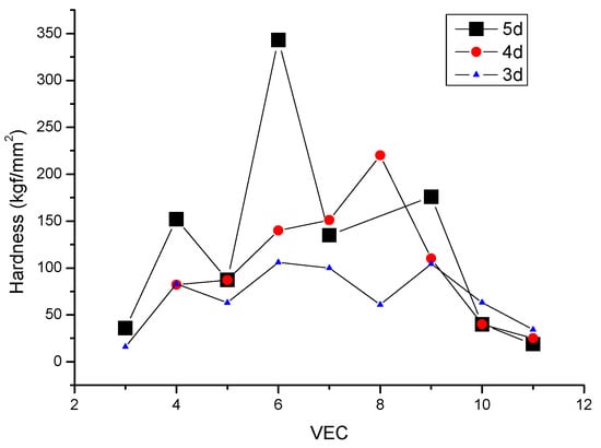
Estimation of Hardness of Single-Phase Metallic Alloys

2.1. The Valence Electron Count (VEC) Dependence of Hardness

To start with, we would like to report on an interesting experimental fact: for single-phase metallic alloys, maximum hardness is attained when the VEC is around 6.5–7. This relationship has long been known for pure metals [8] (see Figure 1), but we have revealed it for two other single-phase systems as well: amorphous metals (see Figure 2) and single-phase high-entropy alloys (HEAs) (see Figure 3). The data for Figure 2 and Figure 3 were collected from our recent published articles [6,7] and from the literature [9,10,11,12,13,14,15,16,17,18,19].

We concentrate on these two single-phase systems, the metallic glasses and HEAs, because, as a first approximation, both can be treated as extended solid solutions. A standard view on metallic glasses is to regard them as very slow liquids with extremely high shear viscosity [20]. In the case of HEAs the high configurational entropy stabilizes the single-phase solid solution’s structure [21].

The understanding of VEC dependence is based on the observation that both hardness and cohesion energy depend on bond strength and both show maximums at a VEC of around 6.5–7 (compare Figure 1, Figure 2, Figure 3 and Figure 4), which corresponds to N_d = VEC-2 = 4.5 ÷ 5 unpaired d electrons. Hardness and cohesion energy show proportional variation as a function of unpaired valence d electrons. The higher the number of unpaired d electrons, the higher the directional bond density. This, together with the isotropic metallic bond density, determines the hardness. The maximum hardness is attained when the VEC is around 6.5–7. This corresponds to 4.5 ÷ 5 d electrons, where 5 is the maximum number of unpaired d electrons.

For the sake of a deeper understanding, we recall here the simple calculation of the textbook Friedel model [22] regarding the dependence of the cohesion energy on the d electron number, N_d. The Friedel model is based on rectangular d band approximation, with a constant density of states D(E) = 5/W (see Figure 5). By integrating D(E), we can obtain the Fermi energy as a function of N_d:

$E_{F} = \frac{W}{10} (N_{d} - 5) + E_{d}$

(1)

Considering E_d = 0 as a reference, we obtain the cohesion energy as:

$E_{c} = 2 \int_{- W / 2}^{E_{F}} E \frac{5}{W} d E = \frac{W}{20} N_{d} (N_{d} - 10) .$

(2)

It turns out that the cohesion energy shows a parabolic dependence on d electron numbers, attaining the maximum for N_d = 5, where W = 5, 7, and 10 eV for the 3d, 4d, and 5d elements, respectively.

Similar parabolic dependence as a function of Nd is found for other cohesion correlated properties. Using the tabulated data from knoledgedoor.com (accessed 20 December 2024) and from [22] we are presenting the VEC dependence of, T_m, the melting point (see Figure 6); γ, the surface energy (see Figure 7); and, more importantly, the elastic properties B, the bulk moduli; E, the elastic moduli; and G, the shear moduli (See Figure 8, Figure 9 and Figure 10).

Due to similar VEC dependencies, these characteristic parameters can also be expressed in terms of their dependence on each other. For example, cohesive energy and surface energy depend on the melting point, as we showed in our recently published article [7]:

$E_{c o h} (k J / m o l) = 0.24 \times T_{m} (K)$

(3)

$γ_{s u r f} (eV) = \frac{T_{m} (K)}{1000}$

(4)

2.2. Estimation of Hardness from Debye Temperature

The strength of interatomic cohesive forces in metals and alloys also manifests itself in the Debye temperature (θ_D(K)), so it can be correlate to the hardness. This relationship was formulated by Deus and Schneider [23]:

$H V = C \cdot {(\frac{k_{B}}{h})}^{2} \frac{A}{V_{m}^{1 / 3}} \cdot θ_{D}^{2}$

(5)

where A is the molar mass, V is the molecular volume, and C is a linear fitted parameter.

Let me note that the formula of Deux and Schneider can also be expressed with the force constant, k, for lattice vibrations. The frequency limit of lattice vibrations is in correlation both to the force constant

k = A ω^{2}

and to the Debye temperature

θ_{D} \cdot k_{B} = ℏ ω

. From these two equations we obtain the force constant:

$k = {(\frac{k_{B}}{ℏ})}^{2} \cdot A \cdot θ_{D}^{2} = 2.86 \cdot 10^{- 5} \cdot A \cdot θ_{D}^{2}$

(6)

The unit of k is N/m (J/m²), and the numerical factor was calculated for normal (tabulated) atomic mass values. Inserting Equation (6) into Equation (5) we obtain hardness as a function of force constant:

$H V = \frac{C}{V_{m}^{1 / 3}} \cdot k$

(7)

On the other hand, the force constant scales with the shear modulus as we have shown in a recent published (see Figure 11) paper [7]. So, we have returned to the well-known hardness–shear modulus relationship in a roundabout way. Nevertheless, all formulas hoping to find the one with least scattering of the data are welcome.

2.3. Estimation of Hardness from Cohesion Energy

Since cohesive energy and hardness showed a similar parabolic dependence on VEC, it is obvious that we should look for a formula to express hardness as a function of cohesive energy. With the help of dimensional analysis, we suggest that HV is proportional to cohesion energy multiplied by electron density, n = Z/V_m, where Z is the metallic valence and V_m is the molar volume. In this way, beside the unpaired d electrons, the sp electrons are also taken into account in determining hardness; so, we propose the following expression:

$H V_{c a l c} = C \cdot E_{c} \frac{Z}{V_{m}},$

(8)

where C is a linear fitted parameter, a constant to be determined; Z is the valence; E_c is in kJ/mol; and V_m is in cm³; then the unit of HV calc is in GPa.

We have found a rather good correlation between the calculated and measured values (see Figure 12), although the measured hardness values published in the literature [6] show a large amount of scatter. Unfortunately, the Ec and Z values also show significant scatter in the literature, this is why we are working on a review paper on the valence electron number and the related electron density values published in the literature. Here, we applied the E_c values published by George Kaptay [24] and the molar volume calculated from the atomic mass (A) and density ρ (V_m = A/ρ) and the Z calculated using the Miedema formula from bulk moduli:

$\begin{array}{l} n = 10^{- 2} \times 6.748 \times \sqrt{\frac{B}{V_{m}}} \\ Z = n \cdot V_{w s} = n \times 1.666 \times V_{m} \end{array} .$

(9)

A normalizing factor C = 1/(100*2.6) adjusts the values to GPa. Finally, the calculated values are obtained in kgf/mm² by multiplying by 100, because 1 GPa = 100 kgf/mm². For high-entropy alloys, all three parameters (Ec, Z, and V_m) can be calculated as a weighted average of the elemental values. Equation (8) permits estimation of the low bound for hardness of any single-phase alloy.

2.4. Estimation of Hardness from Elastic Moduli

Our Formula (8) is a good contribution to the literature [25,26], where various correlations between hardness (HV) and different elastic moduli (bulk, B, shear, G, and elastic, E) or a combination of them have been published. The correlation strongly depends on the type of atomic bonding. In the case of covalent bonding, the correlation is closer than in the case of metallic bonding. For covalent bonding, the following correlations have been found [25]:

B = 10.38 × HV
E = 16.48 × HV
G = 6.78 × HV

(10)

In the case of metallic bonding the correlation of hardness to bulk and Young’s modulus is loose. The best correlation is obtained with the shear modulus, G, which can be understood by the creation and motion of dislocation which are facilitated by shear deformation rather than by volume change. In a recent publication by us [6], this relationship was deduced and tested.

Nevertheless, in the literature one can find many correlations, and it is from there that we have selected the following:

From [26]:

$\begin{array}{l} H = 0.1475 \times G \\ H = 0.0607 \times E \end{array}$

(12)

From [27]:

$H = 0.1769 \times G - 2.899$

(13)

From [29]:

$H V = \frac{G}{B} \frac{E}{6} \frac{1 - 2 ν}{1 + ν} or H = \frac{(1 - 2 ν) B}{6 (1 + ν)}$

(15)

$H = 2 {(k^{2} G)}^{0.585} - 3; k = G / B$

(16)

Formulas (8) and (11) look completely different, but we will show that both depend on the atomic radius (half of the neighboring distance) as, 1/R⁴, and from the metallic valence as Z². Actually, all elastic moduli and hardnesses together represent a density of energy (J/m³), which we identify with the density of bonding energy. As long as the main energy contribution is electrostatic, energy is proportional to 1/R and its density is obtained by dividing it with the atomic volume proportional to R cub; as a result, we obtained the 1/R⁴ dependence. The numerical factor can be debated, but the power dependence cannot.

2.5. The Estimation of Hardness Using the Electrostatic Energy Density of Metallic Bonding

For the sake of a deeper understanding, we recall here the simple calculation from any textbook on electrostatics. We imagine the metal as a regular arrangement of positively charged ions Z, which are neutralized and held together by a common, negatively charged electron sea. The effective shear modulus can be calculated as the second derivative of the total electrostatic energy density:

$G_{e f f} = \frac{τ}{γ} = \frac{α}{R} (\frac{\partial^{2} U_{t}}{\partial d^{2}}),$

(17)

where τ is the shear stress,

γ is the shear strain;

R is the distance between neighboring ions;

α is a geometric factor that depends on the volume fraction of packing, p;

n is the number of nearest neighbors.

Before applying the shear stress, the electrostatic energy is calculated for a sphere-like situation:

$U = - \frac{3}{2} \frac{e^{2} Z^{2}}{d} \cdot 9 \cdot 10^{9},$

(18)

where d = 2 R.

Applying the shear stress, the sphere is deformed to an ellipsoid with the axis:

a = R
b = R(1 − γ/2)
c = R(1 + γ/2)

(19)

and the electrostatic energy will be $U = - \frac{3}{4} \frac{e^{2} Z^{2}}{{(a b c)}^{1 / 3}} \cdot 9 \cdot 10^{9}$ . Dividing this with the atomic volume, we obtain the electrostatic energy density:

$\frac{U}{V} = - \frac{3}{4} \frac{3}{4 π R^{3}} \frac{e^{2} Z^{2}}{{(R^{3} (1 - γ^{2} / 4))}^{1 / 3})}$

(20)

derivative twice, then by neglecting the gamma quadratic terms, we obtain:

$G_{e f f} = \frac{3}{32 π} \frac{e^{2} Z^{2}}{R^{4}} \cdot 9 \cdot 10^{9}$

(21)

In addition to this back-of-an-envelope calculation, much more serious calculations were also carried out; all the more so because of the astrophysical importance of determining the G of the crust of neutron stars.

For such a Coulomb lattice, the elastic constants c′ and c44 were calculated by (Baiko [30,31], and using the Voight, Reuss, and Hill approximations [32], the effective shear modulus G is given [32] by

$G_{e f f} = 0.3462 \frac{n_{N} e^{2} Z^{2}}{2 a} 9 \cdot 10^{9}$

(22)

where $n_{N} = \frac{3}{2 \cdot 4 π {R^{3}}_{w s}}$ is the number density with two atoms/cell and where a is the length of the side of the cubic cell containing two atoms. a = 2R_m, where R_m is the metallic radius, n_N is the number density of the atoms, Z is the valence number of the positive ions, and e is the elementary charge. The factor 9 × 10⁹ appears because we calculate in SI and the result for G is in GPa. In a BCC lattice, R_m = 0.876 × R_ws. Inserting the numerical factors after some algebra, we obtain a formula which depends on two tabulated properties only, the valence Z and the metallic radius, Rm, which are easily accessible in [7] and at www.knowledgedoor.com, accessed on 20 December 2024:

$G = 14 \frac{Z^{2}}{R_{m}^{4}} (GPa),$

(23)

where R is in Å and Z is the valence.

Combining Equation (23) with Equation (11) one obtains the hardness of pure metals as a function of two parameters only: Z and R_m:

$H = 0.234 \frac{Z^{2}}{R_{m}^{4}} (GPa)$

(24)

2.6. Estimation of Hardness Based on Selected Atomic Radius and Metallic Valence Data

Finally, we show that only two parameters are sufficient to estimate the hardness: the atomic radius and the cohesion-based valence. In Formula (24), there are indeed only two parameters, without a third fitting parameter, yet the estimation of the hardness is made difficult by the fact that there are a great many atomic radii and valence tables in the literature and our task now is to select the most suitable ones. For this purpose, we introduce a reference hardness (a norm) for each metal separately, with the help of which we “normalize” the hardness data of the different metals. The reference value is obtained from Formula (24) by keeping the atomic radius of the metal in question, but taking the valence as Z = 1

In Figure 13, we represented the reference values which scatter around 6.5 kgf/mm².

The largest deviations are given by the metals with the smallest (Be) and the largest (Ca) atomic radii. It is clear that the variation in hardness from element to element is caused not by the atomic radius but by the variation in valence. Table 1 summarizes the most commonly used R and Z values for the most common metals.

We need not spend much time discussing the atomic radii, because the radii data collected in the four columns differ little from each other. We have chosen the Goldsmidt data which is obtained after a correction of tabulated atomic radii to the value they would have in a close-packed structure with 12-fold coordination [33].

Before starting the calculations, we make a short compendium of the valence parameters.

Concerning the valence, there are many tables, all showing great differences. In chemistry, the nominal valence is used reflecting an oxidation state. The maximal valency is 8 and is realized, for example, by Osmium in the oxide compound OsO4. Valences given by Trömel [34], show that the d electron of the transition metals could contribute to the valence electrons.

Looking for valence values with more fundamental grounding, we have decided to use the electron density obtainable from ab initio calculations [35]. Conducting calculations for minimizing the electron energy as a function of Wigner–Seitz (WS) radii, one can obtain the numerical value for 4πr²n(r) where r is the WS radii. Using the WS radii, we can determine the electron density, n. Finally, the metallic valence, Z_Vit, is obtained from this n using the Wigner–Seitz volume instead of the atomic volume, Z_Vit = n^x4π(R_ws)³/3.

Rose and Shore [36] have introduced the “bonding valency”, (Z_b), which proved to give quite a good description of the binding energy even for transition metals. The tabulated data of Z_b can also be found in [37].

We can guess that, if we need to calculate a property related to cohesion, we use the valence derived from the cohesive energy, and if we use the formula related to elastic moduli, we use the Z_BM introduced by Miedema, which was calculated based on the bulk modulus. In a recently published article [6], we can find the calculation formulas for the Z-_BM (Equation (5) in [6]) and Z_coh (Equation (8) in [6]) column data. We should also mention that the corrected values of the cohesive energy were taken from G. Kaptay’s article [24].

The best correlation between the calculated and measured hardness data is obtained for Z_coh (see Figure 14).

From the reference and measured hardnesses, an effective valence can be calculated, which shows a close correlation with the Z_coh and Z_BM data (see Figure 15) but correlates poorly with the other three datasets (Z_Vit, Z_bond, and Z_Trö). The explanation is that the hardness is closely related to the cohesive property.

Source link

Ottó K. Temesi www.mdpi.com

Greenberg News

Estimation of Hardness of Single-Phase Metallic Alloys

2.1. The Valence Electron Count (VEC) Dependence of Hardness

2.2. Estimation of Hardness from Debye Temperature

2.3. Estimation of Hardness from Cohesion Energy

2.4. Estimation of Hardness from Elastic Moduli

2.5. The Estimation of Hardness Using the Electrostatic Energy Density of Metallic Bonding

2.6. Estimation of Hardness Based on Selected Atomic Radius and Metallic Valence Data

Greenberg

2.1. The Valence Electron Count (VEC) Dependence of Hardness

2.2. Estimation of Hardness from Debye Temperature

2.3. Estimation of Hardness from Cohesion Energy

2.4. Estimation of Hardness from Elastic Moduli

2.5. The Estimation of Hardness Using the Electrostatic Energy Density of Metallic Bonding

2.6. Estimation of Hardness Based on Selected Atomic Radius and Metallic Valence Data

Related Posts

Residential propane price increases

Environmental Factor – April 2021: Disaster research response experts share insights for pandemic

Materials, Vol. 18, Pages 657: First-Principles Understanding of Mono- and Dual-Emissions in AZnOS:Bi3+ (A = Ba, Ca) Phosphors

Greenberg