Existence of Solutions to the Variable Order Caputo Fractional Thermistor Problem

1. Introduction

A thermistor, the name being a blend of the words “thermal” and “resistor”, is a resistor whose resistance changes with temperature [1,2,3,4]. As can be seen from the references in this paper, during the last two decades, a number of researchers (see [1,2,3,4,5,6,7,8,9,10,11,12,13,14,15,16,17,18]) have studied the complexities of the thermistor problem. Their works have included proving the existence and uniqueness of weak solutions to the problem. Some recent work (see [19,20,21,22,23,24,25]) has even shifted towards computational approaches to examine the thermistor problem in various mechanical contexts by utilizing techniques such as finite difference [19,20] and finite element methods [21,22]. These models capture the interactions between heat dissipation, electrical conduction, and Joules heat generation; for further physical details, see [5]. Notably, this model integrates thermo-visco-elastic effects, which sets it apart from earlier models. The existence of a unique weak solution to the problem was established in [5] by using regularization, time-retarding, and a fixed-point argument.

Positive temperature coefficient (PTC) thermistors are known for their property of increasing resistance as temperature rises. These components are commonly used in series configurations within circuits and act as current limiters to protect the circuitry by serving as substitutes for fuses. As electrical current flows through a PTC thermistor, it generates a small amount of resistive heat. If the current exceeds a certain threshold, the heat generated surpasses the thermistor’s ability to dissipate it, which then causes the device to heat up. This rise in temperature increases the resistance and creates a feedback loop that further elevates resistance and subsequently reduces current flow.

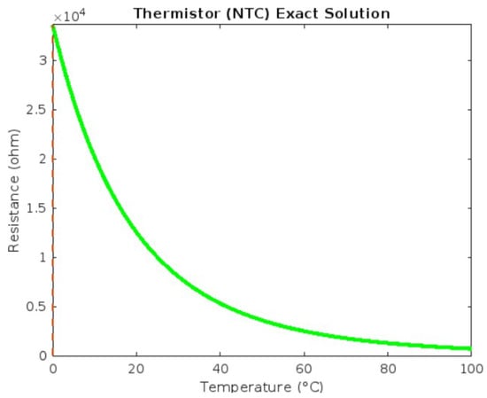
Negative temperature coefficient (NTC) thermistors, which exhibit decreasing resistance with rising temperature, are widely used as temperature sensors in various applications such as fluid temperatures in engine coolants, automotive cabin air, and engine oil. They then transmit these data to control units. In the food processing industry, for example, they ensure optimal temperatures are maintained to prevent spoilage. Additionally, NTC thermistors provide precise temperature regulation in household appliances such as toasters, coffee makers, refrigerators, freezers, and hair dryers. These thermistors come in various physical forms, including axial-loaded glass-encapsulated diodes, epoxy-coated versions with insulated lead wires, cylindrical rods, and disk-shaped configurations, all to meet various application needs. The versatility and reliability of NTC thermistors make them essential in a wide range of temperature sensitive systems and applications across various industries. Their precise measurement and response to temperature changes are crucial for thermal management, temperature control, and temperature sensing applications.

Ammi and Torres [6] investigated the behavior of NTC thermistors and proved the existence and uniqueness of positive solutions to fractional Riemann–Liouville nonlocal thermistor problems on an arbitrary time scale. This research enhanced the mathematical modeling and the understanding of NTC thermistors by providing insights that can inform the design, optimization, and implementation of these components in diverse engineering and scientific fields.

In [7], local and global existence results were established for nonlocal thermistor problems involving a Caputo fractional derivative. The research in [8] resulted in a tube solution to a nonlocal thermistor problem containing conformable fractional derivatives by using fixed-point theory. Shi and Yang [22], analyzed superclose and superconvergence properties of a nonlinear Caputo fractional thermistor problem using a bilinear finite element method. Vivek et al. [9] explored the dynamics and Ulam stability of thermistor problems involving a Hilfer fractional derivative by employing Schauder’s fixed point theorem.

Motivated by these studies, Mazzouz and Henderson [4] investigated the existence and uniqueness of solutions to the Caputo–Katugampola fractional thermistor problem,

$\{\begin{matrix} {}^{c}D^{ı . ℘} ¥ (≀) = \frac{λ ℵ (≀, ¥ (≀))}{{(\int_{υ_{1}}^{υ_{2}} ℵ (♭, ¥ (♭)) d ♭)}^{2}}, \\ ı > 0, 0 < ℘ < 1, ≀ \in J = [υ_{1}, υ_{2}], υ_{1} \geq 0, \\ ¥ (υ_{1}) = ¥_{υ_{1}} \in R, \end{matrix}$

(1)

where
${}^{c}D^{ı . ℘}$ is the Caputo–Katugampola fractional derivative of order ℘, ¥ describes the temperature distribution within a conductor over time ≀, ℵ denotes the electrical conductivity, and
$λ$ is a parameter.

In this paper, we apply fixed-point techniques to investigate the existence and uniqueness of solutions to the variable order Caputo fractional thermistor problem,

$\{\begin{matrix} {}^{c}D^{℘ (≀)} ¥ (≀) = \frac{λ ℵ (≀, ¥ (≀))}{{(\int_{υ_{1}}^{υ_{2}} ℵ (♭, ¥ (♭)) d ♭)}^{2}}, \\ 0 < ℘ (≀) < 1, ≀ \in J = [υ_{1}, υ_{2}], υ_{1} \geq 0, \\ ¥ (υ_{1}) = ¥_{υ_{1}} \in R . \end{matrix}$

(2)

Here,
${}^{c}D^{℘ (≀)}$ is a variable order Caputo fractional derivative of order
$℘ (≀)$ , ¥ represents the temperature distribution within a conductor over time ≀, ℵ is the electrical conductivity, and
$λ$ is a parameter.

Problems involving variable order fractional operators are very useful in other situations such as in viscoelasticity in which the parameters depend on the temperature variation.

Our paper is structured as follows. In Section 2, we review essential definitions and notation for this study. Section 3 contains our main findings. Section 5 contains an example with numerical simulations of our results.

3. Main Results

This section contains the main results of our research. Our first goal is to obtain an integral representation for a solution to our problem. We first need to point out that
$[K (≀)] = 0$ so that in what follows,
$n = [K (≀)] + 1 = 1$ .

Take

$P = [υ_{1}, ≀_{1}], (≀_{1}, ≀_{2}], (≀_{2}, ≀_{3}], \dots, (≀_{k - 1}, υ_{2}]$

to be a partition of the interval
$[υ_{1}, υ_{2}]$ , and consider the function
$℘ (≀) : [υ_{1}, υ_{2}] \mapsto (0, 1)$ that is piecewise constant with respect to
$P$ ; this function is defined as

$℘ (≀) = \sum_{ı = 1}^{k} ℘_{ı} χ_{ı} (≀), for ≀ \in [υ_{1}, υ_{2}],$

where
$0 < ℘_{ı} < 1$ for each
$ı = 1, 2, \dots, k$ , and the constants
$℘_{ı}$ are defined over the intervals specified by
$P$ . Here,
$χ_{ı}$ denotes the indicator (characteristic) function for the interval
$[≀_{ı - 1}, ≀_{ı}]$ , where
$≀_{0} = υ_{1}$ ,
$≀_{k} = υ_{2}$ , and is defined by

$χ_{ı} (≀) = \{\begin{matrix} 1, & if ≀ \in [≀_{ı - 1}, ≀_{ı}], \\ 0, & otherwise . \end{matrix}$

Thus, in view of Definition 4,

$\begin{matrix} {}^{c}D^{℘ (≀)} ¥ (≀) & = \frac{1}{Γ (1 - \sum_{ı = 1}^{k} ℘_{ı} χ_{ı} (≀))} \int_{υ_{1}}^{≀} {(≀ - s)}^{1 - \sum_{ı = 1}^{k} ℘_{ı} χ_{ı} (≀) - 1} \frac{d}{d s} (¥ (s)) d s \\ = \frac{1}{Γ (1 - \sum_{ı = 1}^{k} ℘_{ı} χ_{ı} (≀))} \int_{υ_{1}}^{≀} {(≀ - s)}^{1 - \sum_{ı = 1}^{k} ℘_{ı} χ_{ı} (≀) - 1} ¥^{'} (s) d s \\ = \frac{λ ℵ (≀, ¥ (≀))}{{(\int_{υ_{1}}^{υ_{2}} ℵ (♭, ¥ (♭)) d ♭)}^{2}} . \end{matrix}$

(8)

for
$0 \leq υ_{1} \leq ≀ \leq υ_{2} < + \infty$ . We denote by
$Z_{ı} = C ([≀_{ı - 1}, ≀_{ı}], R),$ the class of functions that form a Banach space with the norm

${∥ ¥ ∥}_{Z_{ı}} = sup_{≀ \in [≀_{ı - 1}, ≀_{ı}]} : i \in 1, 2, \dots, k .$

For each

i \in 2, \dots, k

, let the functions

{\hat{¥}}_{i} \in Z_{i}

be such that

{\hat{¥}}_{ı} (≀) = 0

for all

≀ \in [υ_{1}, ≀_{i - 1}]

. Therefore, in the interval

[υ_{1}, ≀_{1}]

we have

${}^{c}D^{℘_{1}} \hat{¥} (≀) = \frac{1}{Γ (1 - ℘_{1})} \int_{υ_{1}}^{≀} {(≀ - s)}^{℘_{1}} {\hat{¥}}^{'} (s) d s = \frac{λ ℵ (≀, ¥ (≀))}{{(\int_{υ_{1}}^{≀} ℵ (♭, \hat{¥} (♭)) d t)}^{2}} .$

(9)

In the interval
$(≀_{1}, ≀_{2}],$

${}^{c}D^{℘_{2}} \hat{¥} (≀) = \frac{1}{Γ (1 - ℘_{2})} \int_{≀_{1}}^{≀} {(≀ - s)}^{℘_{2}} {\hat{¥}}^{'} (s) d s = \frac{λ ℵ (≀, ¥ (≀))}{{(\int_{≀_{1}}^{≀} ℵ (♭, \hat{¥} (♭)) d t)}^{2}} .$

(10)

In general, in
$(≀_{ı - 1}, ≀_{ı}]$ , we have

${}^{c}D^{℘_{ı}} \hat{¥} (≀) = \frac{1}{Γ (1 - ℘_{ı})} \int_{≀_{ı - 1}^{+}}^{≀} {(≀ - s)}^{℘_{ı}} {\hat{¥}}^{'} (s) d s = \frac{λ ℵ (≀, ¥ (≀))}{{(\int_{≀_{ı - 1}^{+}}^{≀} ℵ (♭, \hat{¥} (♭)) d t)}^{2}} .$

(11)

Consequently, for each
$ı \in 1, 2, \dots, k$ , we examine the auxiliary constant-order initial value problem

$\{\begin{matrix} {}^{c}D^{℘_{ı}} \hat{¥} (≀) = \frac{λ ℵ (≀, ¥ (≀))}{{(\int_{≀_{ı - 1}^{+}}^{≀} ℵ (♭, \hat{¥} (♭)) d t)}^{2}}, ≀_{ı - 1} < ≀ < ≀_{ı}, \\ \hat{¥} (υ_{1}) = {\hat{¥}}_{υ_{1}} . \end{matrix}$

(12)

Definition 6.

We define the solution of problem (2) to be ¥ if there exist functions

¥_{i}

such that

¥_{1} \in Z_{1}

satisfies (9) and

¥_{1} (υ_{1}) = ¥_{1} (≀_{0}) = {\hat{¥}}_{υ_{1}}

;

¥_{2} \in Z_{2}

satisfies (10) and

¥_{2} (≀_{0}) = ¥_{2} (≀_{1}) = {\hat{¥}}_{υ_{1}}

; …;

¥_{ı} \in Z_{ı}

satisfies (11) and

¥_{ı} (≀_{ı - 1}) = ¥_{ı} (≀_{ı}) = {\hat{¥}}_{υ_{1}}

for

ı = 3, \dots, k

Remark 2.

We say that problem (2) possesses a unique solution in

C ([υ_{1}, υ_{2}], R)

if the functions

{\hat{¥}}_{i}

are unique for each

i \in 1, 2, \dots, k

Lemma 2.

For

ı \in 1, 2, \dots, k

, the function

{\hat{¥}}_{i}

is a solution of (12) if and only if it satisfies the integral equation

${\hat{¥}}_{i} (≀) = {\hat{¥}}_{υ_{1}} + \frac{1}{Γ (℘_{i})} \int_{≀_{i - 1}}^{≀} {(≀ - s)}^{℘_{i - 1}} ℏ (s) d s .$

(13)

for
$≀ \in (≀_{i - 1}, ≀_{i}]$ for each
$i \in 1, 2, \dots, k$ .

Proof.

Given that

\hat{¥}

satisfies (12), we rewrite (12) as the equivalent integral equation as follows: For

≀_{ı - 1} < ≀ < ≀_{ı}

, by Lemma 1,

$I_{≀^{+}}^{℘_{ı}} {}^{c}D_{≀^{+}}^{℘_{ı}} ¥ (≀) = I_{≀^{+}}^{℘_{ı}} ℏ (≀) + ρ_{0},$

where

$ℏ (≀) = \frac{λ ℵ (≀, \hat{¥} (≀))}{{(\int_{υ_{1}}^{υ_{2}} ℵ (♭, ¥ (♭)) d ♭)}^{2}} .$

Using the boundary conditions
$\hat{¥} (υ_{1}) = {\hat{¥}}_{υ_{1}}$ , we obtain

$\hat{¥} (≀) = {\hat{¥}}_{υ_{1}} + \frac{1}{Γ (℘_{ı})} \int_{≀_{ı - 1}}^{≀} {(≀ - s)}^{℘_{ı} - 1} ℏ (s) d s .$

(14)

□

For the sake of brevity, we set

$N_{≀}^{℘_{ı}} (s) = \frac{{(≀ - s)}^{℘_{ı} - 1}}{Γ (℘_{ı})} and ℵ_{\hat{¥}} (≀) = ℵ (≀, \hat{¥} (≀)) .$

It is easy to verify that

$\int_{υ_{1}}^{≀} N_{≀}^{℘_{ı}} (s) d s \leq \int_{υ_{1}}^{υ_{2}} N_{υ_{2}}^{℘_{ı}} (s) d s = \frac{{(υ_{2} - υ_{1})}^{℘_{ı}}}{Γ (℘_{ı} + 1)} = N^{*} .$

Prior to presenting our primary findings, we list the following hypotheses that are needed in our analysis.

$(C_{1})$: ℵ is continuous;
$(C_{2})$: $| ℵ_{{\hat{¥}}_{2}} (≀) - ℵ_{{\hat{¥}}_{1}} (≀) | \leq k | {\hat{¥}}_{2} - {\hat{¥}}_{1} |$ ,
$k > 0$ , for all
$≀ \in J$ and
${\hat{¥}}_{1}, {\hat{¥}}_{2} \in R$ ;
$(C_{3})$: $0 < c \leq ℵ_{\hat{¥}} (≀)$ , for all
$≀ \in J$ and
$\hat{¥} \in R$ ;
$(C_{4})$: For
$i = 1, 2, \dots, k$
$\frac{|{\hat{¥}}_{υ_{1}}| {(c (≀_{ı} - ≀_{ı - 1}))}^{2} + λ N^{*} ℵ_{0}^{*}}{{(c (≀_{ı} - ≀_{ı - 1}))}^{2} - λ N^{*} k} < δ_{i} .$

Theorem 2.

Assume that conditions

(C_{1})

–

(C_{4})

hold. Then, the boundary value problem (2) possesses at least one solution in

C ([υ_{1}, υ_{2}], R)

Proof.

Consider the mapping

G_{i} : Z_{ı} \to Z_{ı}

given by

$(G_{i} \hat{¥}) (≀) = {\hat{¥}}_{υ_{1}} + λ \int_{≀_{ı - 1}}^{≀} \frac{ℵ_{\hat{¥}} (s) N_{≀}^{℘_{ı}} (s)}{{(\int_{≀_{i - 1}}^{≀_{i}} ℵ_{\hat{¥}} (♭) d ♭)}^{2}} d s .$

(15)

Let the ball
$B_{δ_{ı}} = \hat{¥} \in Z_{ı} : ∥ \hat{¥} ∥_{Z_{ı}} \leq δ_{ı}$ be the nonempty, closed, bounded, convex subset of
$Z_{ı}$ , where

$δ_{ı} \geq \frac{|{\hat{¥}}_{υ_{1}}| + \frac{λ N^{*} ℵ_{0}^{*}}{{(c (≀_{ı} - ≀_{ı - 1}))}^{2}}}{1 - \frac{λ N^{*} k}{{(c (≀_{ı} - ≀_{ı - 1}))}^{2}}} .$

The proof will be given through several claims.

Claim 1: The function

G_{i}

is continuous for each

i \in 1, 2, \dots, k

. Suppose that

{\hat{¥}}_{m}

is a sequence such that

{\hat{¥}}_{m} \to \hat{¥}

B_{δ_{i}}

. For each

i \in 1, 2, \dots, k

and for every

≀ \in [≀_{i - 1}, ≀_{i}]

, we have

$\begin{matrix} |(G_{i} \hat{¥_{m}}) (≀) - (G_{i} \hat{¥}) (≀)| & \leq λ \int_{≀_{ı - 1}}^{≀} N_{≀}^{℘_{i}} (s) |\frac{ℵ_{{\hat{¥}}_{m}} (s)}{{(\int_{≀_{i - 1}}^{≀_{i}} ℵ_{{\hat{¥}}_{m}} (♭) d ♭)}^{2}} - \frac{ℵ_{\hat{¥}} (s)}{{(\int_{≀_{i - 1}}^{≀_{i}} ℵ_{\hat{¥}} (♭) d ♭)}^{2}}| d s \\ \leq λ \int_{≀_{ı - 1}}^{≀} N_{≀}^{℘_{ı}} (s) [|\frac{ℵ_{{\hat{¥}}_{m}} (s) - ℵ_{\hat{¥}} (s)}{{(\int_{≀_{ı - 1}}^{≀_{ı}} ℵ_{{\hat{¥}}_{m}} (♭) d ♭)}^{2}}| \\ + |\frac{ℵ_{\hat{¥}} (s)}{{(\int_{≀_{ı - 1}}^{≀_{ı}} ℵ_{{\hat{¥}}_{m}} (♭) d ♭)}^{2}} - \frac{ℵ_{\hat{¥}} (s)}{{(\int_{≀_{ı - 1}}^{≀_{ı}} ℵ_{\hat{¥}} (♭) d ♭)}^{2}}|] d s \\ \leq λ \int_{≀_{ı - 1}}^{≀} N_{≀}^{℘_{ı}} (s) [\frac{k | {\hat{¥}}_{m} (s) - \hat{¥} (s) |}{{(\int_{≀_{ı - 1}}^{≀_{ı}} ℵ_{{\hat{¥}}_{m}} (♭) d ♭)}^{2}} \\ + |\frac{{(\int_{≀_{ı - 1}}^{≀_{ı}} ℵ_{{\hat{¥}}_{m}} (♭) d ♭)}^{2} - {(\int_{≀_{ı - 1}}^{≀_{ı}} ℵ_{\hat{¥}} (♭) d ♭)}^{2}}{{(\int_{≀_{ı - 1}}^{≀_{ı}} ℵ_{{\hat{¥}}_{m}} (♭) d ♭)}^{2} {(\int_{≀_{ı - 1}}^{≀_{ı}} ℵ_{\hat{¥}} (♭) d ♭)}^{2}}| | ℵ_{\hat{¥}} (s) |] d s \\ \leq \frac{λ}{{(c (≀_{ı} - ≀_{ı - 1}))}^{2}} \int_{≀_{i - 1}}^{≀} N_{≀}^{℘_{ı}} (s) [k | {\hat{¥}}_{m} (s) - \hat{¥} (s) | \\ + \frac{(k ∥ \hat{¥} ∥_{Z_{ı}} + ℵ_{0}^{*})}{{(c (≀_{ı} - ≀_{ı - 1}))}^{4}} ({(\int_{≀_{ı - 1}}^{≀_{ı}} ℵ_{{\hat{¥}}_{m}} (♭) d ♭)}^{2} - {(\int_{≀_{ı - 1}}^{≀_{ı}} ℵ_{\hat{¥}} (♭) d ♭)}^{2})] d s \\ \leq λ \int_{≀_{i - 1}}^{≀} N_{≀}^{℘_{ı}} (s) [\frac{k | {\hat{¥}}_{m} (s) - \hat{¥} (s) |}{{(c (≀_{i} - ≀_{i - 1}))}^{2}} + \frac{k ∥ \hat{¥} ∥_{Z_{ı}} + ℵ_{0}^{*}}{{(c (≀_{ı} - ≀_{ı - 1}))}^{4}} \\ \times |{(\int_{≀_{ı - 1}}^{≀_{ı}} ℵ_{{\hat{¥}}_{m}} (♭) d ♭)}^{2} - {(\int_{≀_{ı - 1}}^{≀_{ı}} ℵ_{\hat{¥}} (♭) d ♭)}^{2}|] d s \\ \leq \frac{λ}{{(c (≀_{ı} - ≀_{ı - 1}))}^{2}} \int_{≀_{ı - 1}}^{≀} N_{≀}^{℘_{ı}} (s) [k | {\hat{¥}}_{m} (s) - \hat{¥} (s) | + \frac{k ∥ \hat{¥} ∥_{Z_{ı}} + ℵ_{0}^{*}}{{(c (≀_{ı} - ≀_{ı - 1}))}^{2}} \\ \times |(\int_{≀_{ı - 1}}^{≀_{ı}} ℵ_{{\hat{¥}}_{m}} (♭) d ♭ - \int_{≀_{ı - 1}}^{≀_{ı}} ℵ_{\hat{¥}} (♭) d ♭) (\int_{≀_{ı - 1}}^{≀_{ı}} ℵ_{{\hat{¥}}_{m}} (♭) d ♭ + \int_{≀_{ı - 1}}^{≀_{ı}} ℵ_{\hat{¥}} (♭) d ♭)|] d s \\ \leq \frac{λ}{{(c (≀_{ı} - ≀_{ı - 1}))}^{2}} \int_{≀_{i - 1}}^{≀} N_{≀}^{℘_{ı}} (s) \\ \times [k | {\hat{¥}}_{m} (s) - \hat{¥} (s) | + \frac{2 {(k ∥ \hat{¥} ∥_{Z_{ı}} + ℵ_{0}^{*})}^{2}}{{(c (≀_{ı} - ≀_{ı - 1}))}^{2}} \int_{≀_{ı - 1}}^{≀_{ı}} | ℵ_{{\hat{¥}}_{m}} (♭) - ℵ_{\hat{¥}} (♭) | d ♭] d s \\ \leq \frac{λ k}{{(c (≀_{ı} - ≀_{ı - 1}))}^{2}} \int_{≀_{ı - 1}}^{≀} N_{≀}^{℘_{ı}} (s) (1 + \frac{2 {(k ∥ \hat{¥} ∥_{Z_{ı}} + ℵ_{0}^{*})}^{2}}{c^{2}}) |{\hat{¥}}_{m} (s) - \hat{¥} (s)| d s \\ \leq \frac{λ k (c^{2} + 2 {(k ∥ \hat{¥} ∥_{Z_{ı}} + ℵ_{0}^{*})}^{2})}{{(c^{2} (≀_{ı} - ≀_{ı - 1}))}^{2}} \int_{≀_{i - 1}}^{≀} N_{≀}^{℘_{ı}} (s) |{\hat{¥}}_{m} (s) - \hat{¥} (s)| d s \\ \leq \frac{λ k (c^{2} + 2 {(k ∥ \hat{¥} ∥_{Z_{ı}} + ℵ_{0}^{*})}^{2}) N^{*}}{{(c^{2} (≀_{ı} - ≀_{ı - 1}))}^{2}} |{\hat{¥}}_{m} (s) - \hat{¥} (s)| . \end{matrix}$

Since
${\hat{¥}}_{m} \to \hat{¥}$ and ℵ is continuous, the right-hand side of the above inequality tends to zero as
$m \to + \infty$ . Therefore,

$∥ (G_{i} \hat{¥}) (≀) - (G_{i} \hat{¥}) (≀) ∥_{Z_{ı}} \to 0 as m \to + \infty,$

and so
$G_{i}$ is continuous.

Claim 2: For each

i \in 1, 2, \dots, k

G (B_{δ_{ı}}) \subset B_{δ_{ı}}

. We have

$\begin{matrix} |(G \hat{¥}) (≀)| & = |{\hat{¥}}_{υ_{1}} + λ \int_{≀_{ı - 1}}^{≀} \frac{ℵ_{\hat{¥}} (s) N_{≀}^{℘_{ı}} (s)}{{(\int_{≀_{ı - 1}}^{≀_{ı}} ℵ_{\hat{¥}} (♭) d ♭)}^{2}} d s| \\ \leq |{\hat{¥}}_{υ_{1}}| + λ \int_{≀_{ı - 1}}^{≀} \frac{|ℵ_{\hat{¥}} (s)| N_{≀}^{℘_{ı}} (s)}{{(\int_{≀_{ı - 1}}^{≀_{ı}} ℵ_{\hat{¥}} (♭) d ♭)}^{2}} d s \\ \leq |{\hat{¥}}_{υ_{1}}| + \frac{λ}{{(c (≀_{ı} - ≀_{ı - 1}))}^{2}} \int_{≀_{ı - 1}}^{≀} (| ℵ_{\hat{¥}} (s) - ℵ_{0} (s) | + | ℵ_{0} (s) |) N_{≀}^{℘_{ı}} (s) d s \\ \leq |{\hat{¥}}_{υ_{1}}| + \frac{λ (k ∥ \hat{¥} ∥_{Z_{ı}} + {max}_{≀_{ı} \in j} | ℵ_{0} (s) |)}{{(c (≀_{ı} - ≀_{ı - 1}))}^{2}} \int_{≀_{ı - 1}}^{≀} N_{≀}^{℘_{ı}} (s) d s \\ \leq |{\hat{¥}}_{υ_{1}}| + \frac{λ (k ∥ \hat{¥} ∥_{Z_{ı}} + {max}_{≀_{ı} \in j} | ℵ_{0} (s) |)}{{(c (≀_{ı} - ≀_{ı - 1}))}^{2}} \int_{≀_{ı - 1}}^{≀} N_{≀}^{℘_{ı}} (s) d s \\ \leq |{\hat{¥}}_{υ_{1}}| + \frac{λ N^{*} (k ∥ \hat{¥} ∥_{Z_{ı}} + ℵ_{0}^{*})}{{(c (≀_{ı} - ≀_{ı - 1}))}^{2}} \leq δ_{i}, \end{matrix}$

where
$ℵ_{0}^{*} = {max}_{≀_{ı} \in j} | ℵ_{0} (s) |$ , which proves the claim.

Claim 3: $G_{i}$ is relatively compact for each
$i \in 1, 2, \dots, k$ . From Claim 2,
$G_{i} (B_{δ ı}) \subset B_{δ ı}$ , so
$G_{i} (B_{δ ı})$ is uniformly bounded. It remains to show the equicontinuity of
$G_{i}$ for each
$i \in 1, 2, \dots, k$ .

Consider

≀_{1}

≀_{2} \in (≀_{i - 1}, ≀_{i}]

. Then,

$\begin{matrix} |(G_{i} \hat{¥}) (≀_{2}) - & (G_{i} \hat{¥}) (≀_{1})| = |λ \int_{≀_{ı - 1}}^{≀_{2}} \frac{ℵ_{\hat{¥}} (s) N_{≀_{2}}^{℘_{ı}} (s)}{{(\int_{≀_{i - 1}}^{≀_{i}} ℵ_{\hat{¥}} (♭) d ♭)}^{2}} d s - λ \int_{≀_{ı - 1}}^{≀_{1}} \frac{ℵ_{\hat{¥}} (s) N_{≀_{1}}^{℘_{ı}} (s)}{{(\int_{≀_{i - 1}}^{≀_{i}} ℵ_{\hat{¥}} (♭) d ♭)}^{2}} d s| \\ \leq λ \int_{≀_{ı - 1}}^{≀_{2}} \frac{|ℵ_{\hat{¥}} (s)| N_{≀_{2}}^{℘_{ı}} (s)}{{(\int_{≀_{i - 1}}^{≀_{i}} ℵ_{\hat{¥}} (♭) d ♭)}^{2}} d s - λ \int_{≀_{ı - 1}}^{≀_{1}} \frac{|ℵ_{\hat{¥}} (s)| N_{≀_{1}}^{℘_{ı}} (s)}{{(\int_{≀_{i - 1}}^{≀_{i}} ℵ_{\hat{¥}} (♭) d ♭)}^{2}} d s \\ \leq \frac{λ}{{(c (≀_{ı} - ≀_{ı - 1}))}^{2}} (\int_{≀_{ı - 1}}^{≀_{2}} |ℵ_{\hat{¥}} (s)| N_{≀_{2}}^{℘_{ı}} (s) d s - \int_{≀_{ı - 1}}^{≀_{1}} |ℵ_{\hat{¥}} (s)| N_{≀_{1}}^{℘_{ı}} (s) d s) \\ \leq \frac{λ}{{(c (≀_{ı} - ≀_{ı - 1}))}^{2}} (\int_{≀_{ı - 1}}^{≀_{1}} |ℵ_{\hat{¥}} (s)| (N_{≀_{2}}^{℘_{ı}} (s) - N_{≀_{1}}^{℘_{ı}} (s)) d s + \int_{≀_{1}}^{≀_{2}} |ℵ_{\hat{¥}} (s)| N_{≀_{1}}^{℘_{ı}} (s) d s) \\ \leq \frac{λ (k ∥ \hat{¥} ∥_{Z_{ı}} + ℵ_{0}^{*})}{{(c (≀_{ı} - ≀_{ı - 1}))}^{2}} (\int_{≀_{ı - 1}}^{≀_{1}} (N_{≀_{2}}^{℘_{ı}} (s) - N_{≀_{1}}^{℘_{ı}} (s)) d s + \int_{≀_{1}}^{≀_{2}} N_{≀_{1}}^{℘_{ı}} (s) d s) \\ \leq \frac{λ (k ∥ \hat{¥} ∥_{Z_{ı}} + ℵ_{0}^{*})}{{(c (≀_{ı} - ≀_{ı - 1}))}^{2}} [2 {(≀_{2} - ≀_{1})}^{℘_{ı}} + {(≀_{1} - ≀_{ı - 1})}^{℘_{ı}} - {(≀_{2} - ≀_{ı - 1})}^{℘_{ı}}] . \end{matrix}$

As
$≀_{1} \to ≀_{2}$ , the right-hand side of the above inequality approaches zero, so the mapping
$G_{i}$ is equicontinuous. Thus, by the Ascoli–Arzelà theorem, the mapping
$G_{i}$ is relatively compact on
$B_{δ_{i}}$ .

Theorem 1 thus ensures that the auxiliary boundary value problem (12) possesses at least one solution in

B_{δ_{i}}

for each

i \in 1, 2, \dots, k

. Consequently, the boundary value problem (2) possesses at least one solution in

C ([υ_{1}, υ_{2}], R)

given by

$¥ (≀) = \{\begin{matrix} ¥_{1} (≀) = \hat{¥} (≀), ≀ \in [υ_{1}, ≀_{1}], \\ ¥_{2} (≀) = \{\begin{matrix} 0, ≀ \in [υ_{1}, ≀_{1}], \\ {\hat{¥}}_{2} (≀), ≀ \in (≀_{1}, ≀_{2}], \end{matrix} \\ ⋮ \\ ¥_{k} (≀) = \{\begin{matrix} 0, ≀ \in [υ_{1}, ≀_{k}], \\ {\hat{¥}}_{n} (≀), ≀ \in (≀_{k - 1}, ≀_{k}], \end{matrix} \end{matrix}$

□

Theorem 3.

Assume that conditions

(C_{1})

and

(C_{2})

hold with

0 < c_{1} \leq ℵ \hat{¥} (≀) < c_{2}

for all

≀ \in J

and

\hat{¥} \in R

. Then, Equation (12) has a unique solution in

[υ_{1}, υ_{2}]

for each

i \in 1, 2, \dots, k

, provided that

$\frac{λ k (c_{1}^{2} + 2 c_{2}^{2}) N^{*}}{{(c_{1}^{2} (≀_{ı} - ≀_{ı - 1}))}^{2}} \leq 1 .$

(16)

Proof.

As in Claim 2 in the proof of Theorem 2, the mapping
$G_{i} : B_{δ_{ı}} \to B_{δ_{ı}}$ is uniformly bounded. It remains to show that
$G_{i}$ is a contraction.

Consider

i \in 1, 2, \dots, k

and let

¥_{i}^{*}, ¥_{i} \in B_{δ_{i}}

. Then,

$\begin{matrix} |(G_{i} ¥_{ı}^{*}) (≀) & - (G_{i} ¥_{ı}) (≀)| = |λ \int_{≀_{ı - 1}}^{≀} \frac{ℵ_{¥_{ı}^{*}} (s) N_{≀}^{℘_{ı}} (s)}{{(\int_{≀_{ı - 1}}^{≀_{ı}} ℵ_{¥_{ı}^{*}} (♭) d ♭)}^{2}} d s - λ \int_{≀_{ı - 1}}^{≀} \frac{ℵ_{¥_{ı}} (s) N_{≀}^{℘_{ı}} (s)}{{(\int_{≀_{ı - 1}}^{≀_{i}} ℵ_{¥_{ı}} (♭) d ♭)}^{2}} d s| \\ \leq λ \int_{≀_{i - 1}}^{≀_{i}} N_{≀}^{℘_{i}} (s) |\frac{ℵ_{¥_{i}^{*}} (s)}{{(\int_{≀_{i - 1}}^{≀_{i}} ℵ_{¥_{i}^{*}} (♭) d ♭)}^{2}} - \frac{ℵ_{¥_{i}} (s)}{{(\int_{≀_{i - 1}}^{≀_{i}} ℵ_{¥_{i}} (♭) d ♭)}^{2}}| d s \\ \leq λ \int_{≀_{i - 1}}^{≀_{i}} N_{≀}^{℘_{i}} (s) |\frac{ℵ_{¥_{i}^{*}} (s) - ℵ_{¥_{i}} (s)}{{(\int_{≀_{i - 1}}^{≀_{i}} ℵ_{¥_{i}^{*}} (♭) d ♭)}^{2}}| + |\frac{ℵ_{¥_{i}} (s)}{{(\int_{≀_{i - 1}}^{≀_{i}} ℵ_{¥_{i}^{*}} (♭) d ♭)}^{2}} - \frac{ℵ_{¥_{i}} (s)}{{(\int_{≀_{i - 1}}^{≀_{i}} ℵ_{¥_{i}} (♭) d ♭)}^{2}}| d s \\ \leq λ \int_{≀_{i - 1}}^{≀} N_{≀}^{℘_{i}} (s) [\frac{k | {¥_{i}}^{*} (s) - ¥ (s) |}{{(\int_{≀_{i - 1}}^{≀_{i}} ℵ_{¥^{*}} (♭) d ♭)}^{2}} \\ + |\frac{{(\int_{≀_{i - 1}}^{≀_{i}} ℵ_{{¥_{i}}^{*}} (♭) d ♭)}^{2} - {(\int_{≀_{i - 1}}^{≀_{i}} ℵ_{¥_{i}} (♭) d ♭)}^{2}}{{(\int_{≀_{ı - 1}}^{≀_{ı}} ℵ_{{¥_{ı}}^{*}} (♭) d ♭)}^{2} {(\int_{≀_{ı - 1}}^{≀_{ı}} ℵ_{¥_{ı}} (♭) d ♭)}^{2}}| | ℵ_{¥_{ı}} (s) |] d s \\ \leq λ \int_{≀_{ı - 1}}^{≀} N_{≀}^{℘_{ı}} (s)[\frac{k | {¥_{ı}}^{*} (s) - ¥_{ı} (s) |}{{(c_{1} (≀_{ı} - ≀_{ı - 1}))}^{2}} \\ + \frac{c_{2}}{{(c_{1} (≀_{ı} - ≀_{ı - 1}))}^{4}} ({(\int_{≀_{ı - 1}}^{≀_{ı}} ℵ_{¥_{ı}^{*}} (♭) d ♭)}^{2} - {(\int_{≀_{ı - 1}}^{≀_{ı}} ℵ_{¥_{ı}} (♭) d ♭)}^{2})] d s \\ \leq \frac{λ}{{(c_{1} (≀_{ı} - ≀_{ı - 1}))}^{2}} \int_{≀_{ı - 1}}^{≀} N_{≀}^{℘_{ı}} (s)[k | ¥_{ı}^{*} (s) - ¥_{ı} (s) | \\ + \frac{c_{2}}{{(c_{1} (≀_{ı} - ≀_{ı - 1}))}^{2}} |(\int_{≀_{ı - 1}}^{≀_{ı}} (ℵ_{¥_{ı}^{*}} (♭) - ℵ_{¥_{ı}} (♭)) d ♭) (\int_{≀_{ı - 1}}^{≀_{ı}} (ℵ_{¥_{ı}^{*}} (♭) + ℵ_{¥_{ı}} (♭)) d ♭)|] d s \\ \leq \frac{λ}{{(c_{1} (≀_{ı} - ≀_{ı - 1}))}^{2}} \int_{≀_{ı - 1}}^{≀} N_{≀}^{℘_{ı}} (s)[k | ¥_{ı}^{*} (s) - ¥_{ı} (s) | \\ + \frac{2 c_{2}^{2}}{c_{1}^{2} (≀_{ı} - ≀_{ı - 1})} |\int_{≀_{ı - 1}}^{≀_{ı}} (ℵ_{¥_{ı}^{*}} (♭) - ℵ_{¥_{ı}} (♭)) d ♭|] d s \\ \leq \frac{λ k}{{(c_{1} (≀_{ı} - ≀_{ı - 1}))}^{2}} \int_{≀_{ı - 1}}^{≀_{ı}} N_{≀}^{℘_{ı}} (s) (1 + \frac{2 c_{2}^{2}}{c_{1}^{2}}) | ¥_{ı}^{*} (s) - ¥_{ı} (s) | d s \\ \leq \frac{λ k (c_{1}^{2} + 2 c_{2}^{2}) N^{*}}{{(c_{1}^{2} (≀_{ı} - ≀_{ı - 1}))}^{2}} {∥ ¥_{ı}^{*} (s) - ¥_{ı} (s) ∥}_{Z_{ı}} . \end{matrix}$

Since (16) holds for each
$i \in 1, 2, \dots, k$ ,
$G_{i}$ is a contraction. By Banach’s fixed-point theorem, it follows that
$G_{i}$ has a unique fixed point that corresponds to a unique solution of Equation (12) in the interval
$(≀_{i}, ≀_{i}]$ for each
$i \in 1, 2, \dots, k$ . In view of Remark 2, the uniqueness of solutions to Equation (2) is obtained. □

5. Discussion

In this paper, the authors examine a variable order fractional Caputo model for thermistors. Thermistors have important applications in engine cooling and automotive cabin air control as well as in many household appliances such as coffee makers, toasters, refrigerators, freezers, and hair dryers. Conditions guaranteeing the existence and uniqueness of solutions are given by an application of Schauder’s fixed-point theorem. An example is included for illustrative purposes.

As pointed out by one of the reviewers, since the Caputo–Katugampola (CK) fractional operator is a generalization of the Caputo fractional operator, proving the existence and uniqueness of solutions to the CK problem also demonstrates it for the Caputo problem.

As was mentioned in the Introduction, problems involving variable order fractional operators can be useful in many other settings. It is hope that the work here will motivate others to explore variable order fracional problems in other types of applications.

Directions for future research include using other fractional derivatives in the model as well as looking at such models that contain impulsive effects.

Source link

John R. Graef www.mdpi.com

Greenberg News

Existence of Solutions to the Variable Order Caputo Fractional Thermistor Problem

1. Introduction

3. Main Results

5. Discussion

Greenberg

1. Introduction

3. Main Results

5. Discussion

Related Posts

A Two-Hour Fetal Glucagon Infusion Stimulates Hepatic Catabolism of Amino Acids in Fetal Sheep

Environmental Factor – August 2020: NIEHS employees unite to support food drive

Insights from the DETECT-AGING Project

Greenberg