3.1. Design of the Force–Thermal Follow-Up Loading Platform
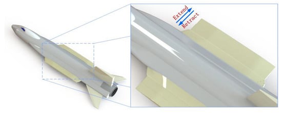
To conduct force–thermal follow-up loading experiments under assessment conditions for deformable wings and enhance the experimental efficiency, this study proposes a design for a force–thermal follow-up loading platform for multi-stage telescopic wings of aircraft. As illustrated in
Figure 11, the system comprises a multi-stage telescopic wing prototype, thermal load application units, force load application units, a supporting platform, and an associated control system. The telescopic wing prototype is mounted on the supporting platform, while the modular thermal and force load units are installed at predesignated positions on the wing surface, aligned with the prototype’s movement direction. A dynamic multi-point distribution equivalence method based on grid reconstruction is proposed to simulate aerodynamic loads. This method equivalently transforms the varying aerodynamic loads during motion into time-varying loads at predefined loading points, enabling follow-up loading throughout the entire process. Both the thermal and force load units are equipped with sensors, such as load cells and thermocouples, to collect real-time loading state data. These sensors connect to the control system, which provides feedback regulation to ensure that the experimental loads accurately follow the predefined loading conditions.
A load unit design analysis is conducted for the multi-stage telescopic wing. Given that the force distribution along the chordwise direction of the wing is nearly uniform, the telescopic wing can be equivalently modeled as a cantilever beam along the spanwise direction, as illustrated in
Figure 12. In this equivalent model, the wing root is assumed to be fixed, while the other end remains free. Corresponding cantilever beam models are established to analyze the structural response under both aerodynamic and concentrated loads.
When the equivalent model is subjected to a uniformly distributed pressure load q, the deflection at the free end (point B), denoted as wB1, is given by the following Equation (1):
where l represents the wingspan, E is the elastic modulus of the material, and I is the moment of inertia of the cross-section.
When the equivalent model is subjected to a concentrated load F, the deflection at the free end (point B), denoted as w
B2, is given by the following Equation (2):
where a represents the distance from the fixed end to the point of load application.
As the number of concentrated loads increases, the accuracy of simulating the uniformly distributed load improves progressively. As shown in
Figure 13, with an increasing number of concentrated loads, the distribution characteristics of shear force and bending moment in the equivalent model more accurately approximate those under a uniformly distributed load. This indicates that increasing the number of concentrated loads within a reasonable range enhances the accuracy of equivalent modeling, thereby providing a more precise representation of the effects of a uniformly distributed load on the structure.
Figure 14 illustrates the variation in deflection error at the free end as the number of equivalent concentrated loads increases. The results indicate that when the number of spanwise concentrated load points reaches four or more, the error reduction rate falls below 2%. Additionally, within the range of [
4,
8] concentrated load points, the equivalent loading error remains below 10%. When the number of spanwise concentrated loads reaches four or more, further increasing the number of concentrated loads reduces the deflection fitting error by less than 2%. Therefore, arranging four or more spanwise loading units meets the acceptable error requirements. Considering the design constraints of the actual drive sources and installation space, four spanwise loading units are selected as the final design configuration.
The number and positions of chordwise loading points are determined through comparative simulation analyses. As shown in
Figure 15, the deformation of 10 characteristic nodes in the fully extended state of the telescopic wing is used as the basis. With 4 spanwise loading units, 4 comparative simulations were conducted for chordwise loading point counts of 3, 6, 9, and 12. These simulations evaluate the deflection deformation under uniformly distributed pressure loads acting on the wing surface. All finite element models were configured identically, differing only in the number of chordwise loading points applied to the wing. The simulation results, presented in
Table 4, indicate that when 36 or more loading points are used, further increases in the number of loading points result in error reduction rates of less than 0.5%. Consequently, 48 loading points are selected as the final configuration.
Based on the design of modular loading units, the aerodynamic loads acting on the wing surface during follow-up loading need to be equivalent to time-varying concentrated loads at predefined loading points. This paper proposes a dynamic multi-point distribution equivalence method for aerodynamic loads, introducing dynamic grid reconstruction to achieve equivalent load simulation under minimum strain energy conditions. Taking the equivalent model of the multi-stage telescopic wing as an example, a grid sensitivity analysis of this method was conducted. The proposed load simulation method was then applied to map the assessment loads onto predefined loading points, resulting in load curves for each loading point throughout the loading process. These results were compared with those obtained using the traditional empirical equal-division method. Finally, an equivalent control system model for the loading units was established. Mechanical and control system models of the designed force–thermal follow-up loading platform were built in simulation software, and simulation analyses were conducted to verify the loading system’s response capabilities.
3.2. Dynamic Multi-Point Distribution Equivalence Method for Aerodynamic Loads
Existing research on load equivalence methods for loading experiments primarily relies on empirical methods, such as equal-area averaging. These methods divide the wing surface into multiple equal-area regions and distribute the aerodynamic loads across these regions, approximating them as concentrated loads to satisfy static equivalence conditions. In contrast, this study adopts the commonly used multi-point distribution method for mapping aerodynamic loads to structural grid points. This method is extended to calculate load equivalence at loading points by incorporating dynamic grid reconstruction, thus proposing the dynamic multi-point distribution equivalence method, which achieves full-process equivalence of time-varying loads.
The basic concept of the multi-point distribution method is as follows: in finite element analysis, after obtaining the aerodynamic loads acting on the wing structure, these loads are mapped from the aerodynamic grid to the structural grid. This is necessary because the grids used for aerodynamic analysis and those for static structural analysis do not perfectly correspond. When the number of structural grid points is sufficiently small, they can be regarded as predefined equivalent loading points.
As shown in
Figure 16, given the position coordinates and corresponding loads of i × k aerodynamic grids on a certain wing surface, the goal is to equivalently transfer all aerodynamic grid loads to predefined loading points{(x
k, y
k), k = 1, 2, 3, …, n}. Taking a particular aerodynamic grid as an example, consider the aerodynamic load po acting on the grid at point o(x
u, y
q). It is assumed that all the predefined loading points and the aerodynamic grid o are connected by a virtual beam (of length l
k), and they both act as cantilever beams with the fixed end at point o. The deformation energy when the load pk is applied to the loading point is as follows:
where EJ represents the bending stiffness of the virtual beam element.
The loads distributed to each structural point should satisfy the following static equilibrium condition:
where k represents the kth loading point, with its value ranging from 1 to n, while n denotes the total number of loading points.
The Lagrangian function is constructed using the method of Lagrange multipliers, as follows:
where , , and are the Lagrange operators for the static equivalent condition construction function, represents the difference in the x-coordinate between loading point k and the aerodynamic grid, and represents the difference in the y-coordinate between loading point k and the aerodynamic grid.
Taking the derivative and setting it equal to zero yields the following:
By combining Formula (3), we can obtain the following:
By solving λ and substituting it into Equation (4), the aerodynamic load of each aerodynamic grid point ouq (u = 1, 2, 3, …, i; q = 1, 2, 3, …, j) is distributed to the corresponding structural grid points. Using the above method, the aerodynamic loads on the wing surface are equivalently allocated to the predefined structural grid points.
The above multi-point distribution method completes the load equivalence of aerodynamic grid loads on the wing surface to the predefined loading points at a specific moment. Building on this, a dynamic multi-point distribution method is proposed by incorporating the mesh reconstruction technique, enabling time-varying loads with changing areas to be equivalently distributed to fixed predefined loading points.
The dynamic multi-point distribution method operates as follows: The entire motion process is discretized into a finite number of time steps at regular intervals, converting the dynamic process into a series of quasi-static processes. At each time step, the aerodynamic grid on the wing surface is re-meshed to achieve dynamic grid updates. The multi-point distribution method is then applied at each time step to allocate the aerodynamic grid loads to the predefined loading points. The loads throughout the discretized process are interpolated and fitted, resulting in the load distribution across all loading points during the motion. This distribution ensures that the equivalent conditions of force and moment are satisfied at all times while minimizing the additional strain energy introduced by load equivalence.
As shown in
Figure 17, during the wing deformation process, the entire process is discretized into t
1 to t
n, representing n finite moments. At each moment, the wing profile undergoes dynamic grid updates. The selection of the time step Δ
t depends on the adopted time discretization strategy, which is typically determined based on the maximum wave speed of the material c
max and the minimum mesh size L
min. In this study, the Courant–Euler–Lagrange (CEL) stability condition is applied, as follows:
This condition ensures the numerical computation remains stable and accurate, allowing for the precise capture of dynamic physical phenomena. To guarantee that the simulation results accurately reflect the real-world physical process, the time step Δt in numerical simulations should be consistent with the characteristic timescale of the physical process.
During the deformation process of the multi-stage telescopic wing, the spanwise length dynamically changes with the deployment state, necessitating an investigation into the influence of mesh size on computational convergence. To address this issue, this study proposes a mesh update strategy based on a fixed total number of mesh elements, ensuring uniformity in mesh distribution throughout the simulation and preventing errors caused by uneven mesh sizes. Since planar meshing is employed in this study, maintaining a constant mesh size across different deployment states would result in varying mesh densities in different regions, potentially affecting computational accuracy. Therefore, instead of fixing the mesh size directly, a strategy of maintaining a constant total number of mesh elements along a specific direction is adopted. This allows the mesh size to adapt dynamically to changes in the spanwise dimension, ensuring consistent meshing across different deformation states. By analyzing the error variations in aerodynamic load calculations under different mesh element counts, the minimum required mesh number for achieving computational convergence is determined. This approach not only guarantees mesh consistency under varying deformation states but also enhances computational efficiency by avoiding unnecessary over-refinement, thereby improving the overall stability and reliability of the numerical simulation.
The sensitivity analysis is performed at the state of t1, with a total of 12 loading points acting on the wing surface. Sensitivity to grid quantity is analyzed separately for chordwise and spanwise directions. The first analysis examines the influence of chordwise grid quantity, and the second analysis examines the influence of spanwise grid quantity.
- (1)
Sensitivity Analysis of Chordwise Grid Quantity
The initial value of the spanwise grid quantity is set to 100, and the chordwise grid quantity is increased from 5 to 300 in increments of 5 to analyze the changes in the load equivalence at the 12 loading points, as shown in
Figure 18. The results indicate that the loading force at each unit becomes nearly unaffected by further increases in the grid quantity once it exceeds 50.
- (2)
Sensitivity Analysis of Spanwise Grid Number
The number of spanwise grids is initially set to 50, and the spanwise grid number is increased from 50 to 3000 in increments of 50. The variations in the load equivalence at 12 loading points are analyzed, as shown in
Figure 19. The loads with significant variations, after the number increases to 1500 or more, show an absolute error of less than 0.2 N when compared to the final convergent value. The force load distribution is almost no longer affected by the change in the number of grids.
Based on the grid sensitivity analysis, the increase in grid number has a certain impact on the load equivalence results. However, once the grid number reaches a certain threshold, the change in grid number has minimal effect on the load equivalence results. Therefore, the grid update method for each moment is to keep the grid unchanged based on a certain number. The chordwise grid length remains unchanged as the wing does not deform in the chordwise direction, while the spanwise grid length gradually increases. In subsequent analyses, the grid reconstruction number is determined to be 50 for the chordwise direction and 1500 for the spanwise direction. In this study, the minimum mesh size L
min is determined to be 0.107 mm, while the maximum wave speed of the selected material GH4169 is calculated as 4901.781 m/s. Consequently, based on the CEL condition, the time step Δ
t required to maintain computational stability is calculated as follows:
3.3. Method Comparison and Validation
3.3.1. Load Calculation
In existing research, a commonly used load equivalence method is to divide the wing surface into multiple equal-area regions, set loading points, and directly distribute the loads based on the total force acting on the wing surface, using the equal-area allocation method. Equation (10) is as follows:
where P represents the pressure load acting on the wing, S denotes the loaded area, and n indicates the number of equally divided area sections. Fi represents the load value assigned to the i-th loading point.
That is, the wing surface is divided into multiple regions of equal area, with a loading point set in each region. The resultant force of the loads at multiple loading points, Fi, is equal to the total load acting on the wing surface, while the position design also considers the equivalence of the moment. This method can somewhat simulate aerodynamic loads that are relatively evenly distributed. However, when applied to complex and variable aerodynamic loads, this method struggles to achieve a good fit. Therefore, one advantage of the dynamic multi-point allocation method studied in this paper is its ability to fit and equivalently simulate complex aerodynamic loads on the wing surface with high accuracy. Similarly, when handling uniformly distributed aerodynamic loads, the method proposed in this paper still maintains a high level of fitting accuracy. Below, using the multi-stage telescopic wing equivalent model as the object, both methods will be applied to compare the fitting accuracy of wing surface load deformation trends to verify the superiority of the method studied in this paper.
First, the variation in wing surface loads during the entire telescopic process of the multi-stage telescopic wing under the 15 kPa test load will be analyzed. When the multi-stage telescopic wing extends, the extension speed is constant, and the change in area per unit time is a fixed value. Under the pressure load, the aerodynamic load on the wing surface increases linearly. The fixed wing area remains constant, while the middle and outer wings extend synchronously. The resultant forces on each wing surface, i.e., F
f, F
m, and F
o, are as follows:
where Sf refers to the loaded area of the fixed wing, Sm denotes the loaded area of the intermediate wing, Sm1 represents the initial loaded area of the intermediate wing, lm is the chord length of the intermediate wing, So refers to the loaded area of the outer wing, So1 represents the initial loaded area of the outer wing, lo is the chord length of the outer wing, and v is the extension speed.
The total aerodynamic force F acting on the wing surface is as follows:
The change curve of the total force acting on the wing surface is shown in
Figure 20.
The aerodynamic load equivalence distribution is performed using both the traditional equal-area division method and the dynamic multi-point allocation method. The results are shown in
Figure 21 and
Figure 22, respectively.
3.3.2. Initial Moment Analysis and Validation
After obtaining the load distribution from both methods, a comparison analysis was conducted by simulating the deformation trend of the wingtip deflection under the equivalent loads and comparing the fitting degree with the aerodynamic load. The constraints for the initial moment analysis at 0 s are shown in
Figure 23. The root of the equivalent wing was fixed, and simulations were carried out under the following three load conditions on the wing surface: ① the evaluation aerodynamic load, ② the equal-area distribution load, and ③ the dynamic multi-point allocation method equivalent load.
The initial moment data of the three load cases were input into the simulation model to obtain the simulation results, as shown in
Figure 24. The wingtip deformation trajectories were extracted from the three results to analyze the fitting effects of different equivalent methods and aerodynamic loads.
Figure 25 shows the extracted wingtip deformation trajectories under the three loading conditions.
To comprehensively evaluate the fitting performance of the proposed dynamic multi-point allocation method and the traditional equal-area allocation method in practical applications, this paper calculates two commonly used error metrics, namely root mean square error (RMSE) and the coefficient of determination (R2), for comparative analysis. RMSE is primarily used to measure the magnitude of fitting errors between the two methods, giving higher penalties to larger errors. R2, on the other hand, reflects the correlation between the model’s calculation results and actual values, indicating the model’s ability to explain data variability. Through the joint analysis of these two metrics, the fitting performance of the model can be more comprehensively assessed.
The root mean square error (RMSE) is a metric used to measure the difference between the fitted values and the true values. It is defined as the square root of the average of the squared differences between the fitted and actual values, as follows:
where ypred,i is the equivalent value for the i-th sample, ytrue,i is the aerodynamic load value, and n is the number of samples in the dataset. A smaller RMSE value indicates that the difference between the model’s fitting results and the actual results is smaller, meaning the fitting performance is better.
The coefficient of determination R
2 measures the correlation between the model’s computed values and the actual values. Its formula is as follows:
where is the mean of the actual values. The R2 value ranges between 0 and 1, with a value closer to 1 indicating a stronger ability of the model to explain the data variability and a better fitting performance. This paper evaluates the superiority of the fitting performance of the two methods by comparing their performance based on RMSE and R2 metrics.
For the error analysis of the two methods at the initial state, RMSE and R
2 values were calculated using the wingtip deflection simulation trajectory data. The fitting error results for the dynamic multi-point allocation method and the equal-area distribution method at the initial moment are shown in
Table 5.
The results show that, at the initial moment, the dynamic multi-point allocation method proposed in this paper outperforms the equal-area distribution method in both metrics. Specifically, the smaller RMSE indicates a better fitting effect, while the R2 value close to 1 for the dynamic multi-point allocation method indicates its excellent fitting performance, which is capable of explaining the variability in the data well.
3.3.3. Continuous Process Analysis and Validation
In practical load equivalence applications, the telescoping wing undergoes a continuous deformation process, requiring the equivalent aerodynamic loads to be applied throughout the entire process. During the equivalence, the entire process is discretized into a finite number of time instances, and the equivalent time-varying load curve for the whole process is fitted. To compare the dynamic process, the method proposed in this paper is contrasted with the traditional empirical method. Several typical working conditions during the entire process are selected for dynamic process comparison, as shown in
Table 6. The selected working conditions include moments when the number of loading points changes and intermediate instances.
For different operating conditions, comparative simulation models are established, with the same constraints as described in the previous section. The load data at different time instances are input into the simulation model, and the results are obtained. The wingtip deformation trajectories are extracted from the three sets of results to analyze the fitting effects of different equivalence methods under aerodynamic load conditions.
Figure 26 shows the extracted wingtip deformation trajectories under the three loading conditions at different time instances.
The RMSE and R
2 values are calculated using the wingtip deflection simulation trajectory data for each operating condition. The fitting error results for the dynamic multi-point distribution method and the area-based distribution method at each time instance are shown in
Table 7.
Figure 27 visualizes the fitting error results at different time instances. From the figure, it can be observed that the dynamic multi-point distribution method proposed in this study outperforms the area-based distribution method in both RMSE and R
2 metrics at all time instances. In terms of RMSE, the dynamic multi-point method slightly outperforms the traditional method in the early stage and continues to maintain a lower error as the wing extends. Meanwhile, the R
2 value of the dynamic multi-point distribution method starts at 0.84 and rapidly approaches 1, maintaining a value close to 1 throughout the wing extension. This indicates that, in the entire equivalence process, the dynamic multi-point method provides a better fit to the aerodynamic loads compared to the area-based method, demonstrating a stronger ability to adapt to the variation in the load.
From the above comparative analysis, it is evident that the two error metrics, namely RMSE and R2, evaluate the methods from different perspectives. RMSE focuses on the absolute difference between the fitted values and the actual values, with lower RMSE values indicating better performance in terms of absolute errors. On the other hand, R2 emphasizes the correlation between the fitted values and the actual values, with higher R2 values indicating that the method can better capture the variability in the data and has a stronger fitting capability.
Through the combined analysis of these two metrics, it can be observed that the area-based distribution method exhibits a relatively high RMSE and a lower R2 value. This suggests that the area-based method may not fully capture the variation in the load distribution in certain cases or that it may involve a significant fitting error. In contrast, the dynamic multi-point distribution method proposed in this study shows better fitting performance, particularly in terms of smaller errors and higher fitting accuracy.
3.4. Force–Thermal Follow-Up Loading System Modeling and Simulation Analysis
To ensure that each force loading unit can apply the preset force–load curve, a force feedback control system is designed for real-time feedback control of the loading unit’s force. The loading units are organized into a modular system, so an equivalent system model is established for a single loading unit.
Figure 28 shows the equivalent impedance control model of the loading unit. The servo cylinder in the follow-up loading unit is simplified and equivalent to a moving slider with the mass m
d, with the driving input F(t) and displacement x
1(t). The loading unit and the deformed wing surface are considered to be in constant contact during the loading process. k
d is the equivalent stiffness of the disc spring in the loading unit, and c
d is the system’s equivalent damping. The theoretical model for the follow-up loading unit is established as follows:
Taking the Laplace transformation of Equation (13), the expression is obtained as follows:
Equation (14) represents the transfer function of the moving slider displacement x1 corresponding to the driving input force F in the deformable wing tracking loading control system, as follows:
Based on the transfer function from Equation (19), the control program block diagram of the tracking loading system is provided, as shown in
Figure 29. The input force F
d serves as the system input, and the equivalent spring force F during the tracking process is the output, which is fed back to the PID controller. The PID controller adjusts the tracking loading unit to ensure the output force follows the desired force. The output of the PID algorithm is shown in Equation (16):
where F(t) is the output of the controller; e(t) is the response error; and Kp, Ki, Kd are the coefficients for the proportional, integral, and derivative terms, respectively.
According to the design scheme of the force–thermal follow-up loading platform, a mechanical system model was established and imported into ADAMS2020. The material properties of each component were defined, appropriate motion pairs and contacts were added at the joints, and the corresponding driving conditions were applied to construct the loading platform mechanical system, as shown in
Figure 30. Combining the established control system model, a control system simulation program block diagram was built. The integrated simulation of the follow-up loading platform with force feedback control was conducted to analyze the loading force error and the stability of the control system.
Figure 31 shows the entire process of dynamic loading. The twelve force loading units of the dynamic loading platform are divided into four rows, with three loading units in each row. The loading units in the same row act on the same section of the wing surface. For the analysis of the loading process, the four rows of loading units are taken as an example from the side view. The dynamic loading process is as follows: In the initial state, the four rows of loading units are positioned away from the external surface of the telescoping wing. During the loading process, the first two rows of loading units apply force to the telescoping wing. As the wing extends, the resultant force from the loading units acting on the wing increases. When the wing extends to the position of the third row of loading units, the third row of loading units rises and makes contact with the external surface of the wing, applying force. Similarly, when the wing extends to the position of the fourth row of loading units, the fourth row of loading units rises to make contact and applies force. This process continues until the wing is fully extended. During retraction, the process is reversed. When the telescoping wing retracts to the corresponding loading unit position, the loading units separate from the wing surface until complete retraction is achieved.
During the dynamic loading process, the resultant force applied by the loading points is equivalent to the resultant force acting on the wing under a uniform pressure load. The load–time curve for each loading unit throughout the entire process can be determined based on the position of each row of loading units and the extension speed of the telescoping wing. The force feedback control system program for each loading unit is shown in the figure. The program mainly adopts the PID control method, specifying the force curve for each loading unit, so that the force feedback control system can apply the specified force to the wing surface of the telescoping wing.
The feedback curve for the given force curve in the force feedback control system is shown in
Figure 32. For a constant force loading system, force control follow-up can be achieved within 0.2 s. For time-varying loads, the loading system can also achieve load follow-up within 0.4 s with good accuracy. Simulation analysis shows that the loading error is within 1%. As seen in the figure, during the deformation process, the applied loading force can stably follow the input force curve.