
2.1. Research Methods
This study collected circuit fault data for 2021, 2022 and 2023, and the average number of faults at different voltages (10 kv, 35 kv, 110 kv, 220 kv and 550 kv) per year was roughly 120,000, 8000, 3000, 900 and 350.
In terms of obtaining and processing fault data, we first obtained the location information, the number of faults and the corresponding fault voltage of each fault area in the research area, also recording the time and type of faults. The processed extreme weather indicator data and power fault data were spatially correlated and matched.
2.1.1. Establishment of Extreme Weather Risk Assessment Model
In the formula, F is the extreme weather disaster risk index, which is used to represent the risk degree. The greater the value, the greater the disaster risk degree is. WHi represents the weight value of the disaster risk index in the extreme meteorological disaster risk assessment model. XHi is the standardized value of each evaluation index.
The extreme weather disaster risk index method is mainly based on the differences in the raster data of the transmission line risk evaluation results of extreme disasters in different research periods. The raster computer in the geographic information software Arcmap is used to calculate the raster data of risk evaluation in different research periods and obtain the risk index change distribution map.
2.1.2. Selection of Extreme Weather Characteristic Indicators
Extreme weather events exist in sharp contrast to average weather events. Beniston and his team identified three criteria that define extreme weather events: low frequency of events; serious social and economic losses; and a relatively small or large strength value. In the third and fourth assessment reports of the IPCC, extreme climate events are clearly defined from the dimensions of the probability distribution, that is, for a specific place and time, extreme climate events are events with a very low probability of occurrence, and their occurrence probability usually only accounts for 10% or less of similar climate events. This definition is concise and precise, and fully takes into account the differences in climate in different regions.
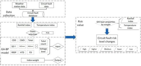
Combined with the above studies on extreme weather indicators by many researchers, this study uses the principal component analysis method to screen out the following extreme weather characteristic indicators as inputs to the neural network model: maximum continuous dry days (CDD), maximum continuous wet days (CWD), total annual precipitation, average annual precipitation intensity (SDII), heavy precipitation days (R25 mm and R50 mm), heavy precipitation rate (R95p), high-temperature days (HTD), and frost days (FD). The characteristics of extreme weather are defined below:
Maximum consecutive dry days (CDD): The maximum number of consecutive days without precipitation in a year.
Maximum consecutive wet days (CWD): The maximum number of consecutive days with precipitation in a year.
Total annual precipitation: The total amount of precipitation in a year.
Average annual precipitation intensity (SDII): The ratio of total annual precipitation to wet days (days with daily precipitation greater than 1 mm).
Heavy precipitation days (R25 mm and R50 mm): Days when the daily precipitation is greater than or equal to 25 mm and 50 mm.
Heavy precipitation rate (R95p): The ratio of annual cumulative precipitation to total annual precipitation when the daily precipitation is greater than 95% of the quantile value.
High-temperature days (HTD): The number of days in the year with a maximum daily temperature of 35 degrees Celsius or higher.
Frost days (FD): The number of days in the year with a minimum daily temperature of 0 °C or less.
2.2. Establishment of Power Grid Fault Risk Grade Evaluation Model Based on GA-BP Neural Network
According to the current research methods for investigating extreme weather events, this research obtained the observation data of extreme weather and the methods of calculating and studying extreme weather of conventional meteorological observation stations. Data and statistics for national meteorological observation stations and meteorological bureaus in the target research area were obtained for the years studied. These data include hourly rainfall, hourly average temperature, hourly maximum temperature, hourly minimum temperature, hourly maximum wind speed, instantaneous wind speed, and average wind speed. The geographical boundary range shp data of the study area were obtained. Meteorological observation stations in the study area provided numerical observation results according to extreme weather research indicators. At the same time, the China Southern Power Grid Company provided the location information, the number of faults and the corresponding fault voltage of each fault area in the study area.
The converted extreme weather indicator data and circuit failure data were spatially correlated and matched, and ArcMap geographic information processing software was used for processing to ensure that the fault data in each study area were matched with the corresponding meteorological data.
The structure of the neural network model for correlation analysis between extreme weather and circuit faults based on the GA-BP algorithm is defined as follows:
To realize construction of the sample set, pre-classification is performed based on the extreme weather index data and circuit fault data. The sample set is divided into training set, verification set and test set to ensure the generalization ability and stability of the model. The definition of extreme weather is mainly based on the pre-classification of indicator data and the data of the fault area, including the number of faults.
The input layer contains nine nodes corresponding to the nine extreme weather indicators: CDD, CWD, total annual precipitation, SDII, R25 mm, R50 mm, R95p, HTD, and FD.
The output layer contains 1 node which is the count of circuit faults divided by different voltages.
The genetic algorithm is responsible for macroscopic search of optimal hyperparameters. The gradient descent of the multi-layer perceptron (MLP) is responsible for micro-adjusting the network weight.
Genetic algorithms are used to optimize neural network parameters (number of hidden layer nodes, regularization parameters, and learning rate) by simulating natural selection (selection, crossover, variation, etc.) to find the best combination of parameters in the search space to minimize the objective function (MSE). The multi-layer perceptron (MLP) uses gradient descent to optimize the weight of the neural network.
The steps for optimizing the initial weight based on the GA-BP algorithm generally include the following: chromosome coding, population initialization, adjustment, fitness function, selection, crossover, variation, and iteration, etc.
The parameters of the neural network model are set as follows: the genetic algorithm sets 1 hidden layer; the number of nodes in the hidden layer has the range [5, 100]; the regularization parameter alpha has the range [0.0001, 0.1]; the initial learning rate has the range [0.0001, 0.1]; and the number of iterations of the genetic algorithm is set to 1000 times. We set the maximum number of iterations of the multi-layer perceptron (MLP) neural network during training to 500, using the non-linear activation function ReLU.
Dropout layers were initially tested but removed due to limited improvement in validation loss, suggesting that the dataset size and regularization parameters were sufficient to prevent overfitting.
The loss function uses the mean square error (MSE) as the loss function, and obtains the lowest MSE by iterating 1000 times, determining the optimal solution of the best number of hidden layer nodes, regularization parameters and learning rate.
In the training process, the initial weight and bias after GA optimization are used as the initial state of the BP neural network. We implement the backpropagation algorithm to further minimize error by adjusting the weight and bias. We use Adam to update the weights. In order to prevent overfitting, the loss of the validation set is monitored, and the training is stopped in advance when the loss no longer decreases.
The dataset is divided into a training set, a validation set, and a test set (80% training, 20% testing).
The model performance is evaluated on the test set using the R2 (coefficient of determination) and MAE (average absolute error) indicators to evaluate the model’s effect.
The importance evaluation of the global weight associated with extreme weather and circuit faults based on the GA-BP neural network is calculated as follows:
After the training is completed, the contribution of each input feature to the output (count of failures) is calculated, and the importance of each weather indicator is assessed by analyzing the post-training weights.
We assume that the 9 nodes in the input layer are X = [x1, x2, x3…, x9], and the hidden layer, they are H = [h1, h2, h3…, hi]. The weight matrix from the input layer to hidden layer is , where represents the weight from input node to hidden layer node.
is the activation function, and is the bias of the hidden layer node . The output layer node is , and the weight matrix from the hidden layer to the output layer is , where represents the weight from the hidden layer node to the output layer node . indicates the offset of the output layer node.
Ci is the total contribution of the input feature to the output Z.
The closer is to 0, the less risky the event is, and the closer is to 1, the more risky the event is. Using this function as a method to calculate the confidence can effectively express the confidence of these kinds of factors.
Through the above steps, the relative importance of each weather index to transmission line faults can be quantified, and the global weight of each input feature can be reflected, which can provide a basis for further decision analysis.
Source link
Jialu Li www.mdpi.com