
1. Introduction
Ordinary least squares (OLS) estimation was used for 39 US states in 2010. It was found that (i) more energy-dense states have less biodiversity, (ii) more expensive energy is associated with a greater preservation of biodiversity, and (iii) the change in direction for greater inequality is also associated with a greater preservation of biodiversity. The Gini index changes cause the most substantially observed effect.
2. Literature Review
The authors first set the stage by introducing the recent literature in the context of a developed country, looking at the biodiversity and energy linkage and then discussing income inequality and environmental outcomes in the United States and other developed countries.
2.1. Biodiversity and Ecology During Energy Transition
However, the interest lies in the energy effect, and the authors consider the pre-transition period and socio-economic impact. Thus, this paper further explores the recent literature regarding total energy consumption and biodiversity.
2.2. Energy and Biodiversity: Consumption and Its Effects
The paper moves forward by looking at the recent trends in the US energy markets.
2.3. Energy Prices and Consumption in the US
2.4. Income Inequality and Environmental Outcomes in the US
The authors of this study suggest that when inequality rises, biodiversity conservation arises because of a structural shift. Due to extreme inequality, there is less industrial expansion in highly unequal regions, indicating lower economic growth and reduced industrialization, which preserves natural biodiversity. When income inequality is rather extreme and there is a wealth concentration, wealthier elites may also push for environmental conservation at home while benefitting from resource exploitation elsewhere. Finally, in regions with high income inequality, state investments in industrial development may be lower, reducing pressure on biodiversity.
To summarize, energy consumption impacts greenhouse gas emissions via, in part, urbanization and farming, which also affect land use change and bio-chemical cycles that have their impacts on biodiversity change. The higher the energy price, the less energy is consumed (although it is deemed inelastic in general), and the less biodiversity change occurs. Regarding income inequality change, the more unequal the state becomes, the more urbanized it becomes, and the more biodiversity change occurs. Therefore, the authors examine the novel addition of Gini index change in conjunction with energy consumption and biodiversity change, which have already been explored. Now, the article proceeds to the empirical estimation of the model.
3. Data and Method
4. Empirical Results
5. Discussion and Implications for Policy
In this study, biodiversity proxied by the state’s protected area percentage was examined based on the energy density of the state, Gini index change, and electricity price. It is found that (i) more energy-dense states have less biodiversity, (ii) more expensive energy is associated with a greater preservation of biodiversity, and (iii) greater inequality is also associated with a greater preservation of biodiversity. The Gini index changes cause the most substantial observed effect.
The results reflect what has been discussed in the literature regarding energy consumption’s detrimental effects on biodiversity. More expensive energy is most likely associated with less consumption, albeit energy is mainly inelastic, feeding into the impact of more preserved biodiversity. Lastly, and surprisingly, an increase in inequality is associated with a greater preservation of biodiversity. As far as the authors know, this last result is not yet documented in the literature.
As for the policy implications regarding energy density and expenditures and their negative relationship with biodiversity protection, stricter environmental regulations may be needed to regulate energy-intensive economic structures or provide incentives for cleaner technologies. As for energy prices, which have a positive relationship with biodiverse area conservation, carbon taxes or energy subsidy reductions could be suggested, making energy-intensive industries less attractive. Lastly, as for income inequality changes, we advise equitable and sustainable development with economic growth or degrowth to achieve biodiversity conservation and the well-being of society.
Regarding limitations, this study’s cross-sectional nature is limited to the dissection of long-term effects. Indeed, this study would benefit from panel data availability, particularly for the income inequality variables. This circumstance implies that, with more data available, a more longitudinal study would be beneficial in dissecting the environment-energy-social nexus.
6. Conclusions
Biodiversity is changing and being lost and projected to be lost in decades, bringing dire consequences to economies. The authors hereby inquire whether energy density and prices can explain biodiversity outcomes in conjunction with income inequality changes.
A relatively focused study for a cross-section of 39 US states was conducted in 2010 using OLS. The findings revealed that (i) more energy-dense states have less biodiversity, (ii) more expensive energy is associated with more preserved biodiversity, and (iii) the change in direction for a greater inequality is also associated with more preserved biodiversity. This study highlights the need for further research into presumably diverse channels that affect income inequality change and biodiverse area conservation. These findings are especially relevant in the face of recent step-backs in environmental regulations in the US.
This research concludes that more investigation should be conducted into presumably diverse channels that affect income inequality change and biodiverse area conservation to bring about novel results and further cement the channels through which inequality affects the environment. For example, the exploration of underlying causal mechanisms could be undertaken, such as the role of conservation policies in high inequality contexts or the influence of interest groups on environmental protection.
Author Contributions
A.A.: Conceptualization, Data curation, Formal analysis, Investigation, Methodology, Visualization, Writing—original draft. J.A.F.: Funding acquisition, Investigation, Methodology, Supervision, Validation, and Writing—review and editing. B.C.: Funding acquisition, Supervision, and Writing—review and editing. S.S.: Funding acquisition, Writing—review and editing. All authors have read and agreed to the published version of the manuscript.
Funding
CeBER’s research is funded by national funds through the FCT—Fundação para a Ciência e a Tecnologia, I.P., through project UIDB/05037/2020, DOI 10.54499/UIDB/05037/2020. This research was also supported by the Association for the Development of Industrial Aerodynamics (ADAI), Associate Laboratory of Energy, Transports and Aeronautics (LAETA), and the Portuguese Foundation for Science and Technology (FCT) through the projects UIDB/50022/2020 (DOI: 10.54499/UIDB/50022/2020), UIDP/50022/2020 (DOI: 10.54499/UIDP/50022/2020) and LA/P/0079/2020 (DOI: 10.54499/LA/P/0079/2020).
Institutional Review Board Statement
Not applicable.
Informed Consent Statement
Not applicable.
Data Availability Statement
Data are available on request from the corresponding author.
Acknowledgments
The first author wishes to acknowledge the Fundação para a Ciência e a Tecnologia (FCT) for supporting her research through the PhD research Grant 2023.01539.BD. Also, the third author wishes to acknowledge the DRIVOLUTION Project—Transição para a fábrica do futuro (7141-02/C05-i01.02/2022.PC644913740-00000022-23)—which was financed by the PRR—Recovery and Resilience Plan—and by the Next Generation EU European Funds, following NOTICE No 02/C05-i01/2022 for supporting his research.
Conflicts of Interest
The authors declare no conflicts of interest.
Appendix A
Table A1.
List of states included in this empirical investigation.
Table A1.
List of states included in this empirical investigation.
| State | Abbreviation | State | Abbreviation |
|---|---|---|---|
| Alabama | AL | Nevada | NV |
| Arkansas | AR | New Hampshire | NH |
| California | CA | New Jersey | NJ |
| Colorado | CO | New Mexico | NM |
| Connecticut | CT | New York | NY |
| Delaware | DE | North Carolina | NC |
| District of Colombia | DC | North Dakota | ND |
| Florida | FL | Ohio | OH |
| Georgia | GA | Oregon | OR |
| Illinois | IL | Pennsylvania | PA |
| Indiana | IN | Rhode Island | RI |
| Iowa | IA | South Carolina | SC |
| Kansas | KS | South Dakota | SD |
| Maine | ME | Tennessee | TN |
| Maryland | MD | Utah | UH |
| Massachusetts | MA | Vermont | VT |
| Michigan | MI | Virginia | VA |
| Minnesota | MN | Washington | WA |
| Montana | MT | Wisconsin | WI |
| Nebraska | NE | Wyoming | WY |
References
- Wei, Y.; Du, M.; Huang, Z. The effects of energy quota trading on total factor productivity and economic potential in industrial sector: Evidence from China. J. Clean. Prod. 2024, 445, 141227. [Google Scholar] [CrossRef]
- Isbell, F.; Gonzalez, A.; Loreau, M.; Cowles, J.; Díaz, S.; Hector, A.; Mace, G.M.; Wardle, D.A.; O’Connor, M.I.; Duffy, J.E.; et al. Linking the influence and dependence of people on biodiversity across scales. Nature 2017, 546, 65–72. [Google Scholar] [CrossRef] [PubMed]
- Koutsandreas, D. A Nexus-Based Impact Assessment of Rapid Transitions of the Power Sector: The Case of Greece. Electricity 2023, 4, 256–276. [Google Scholar] [CrossRef]
- Li, Y.; Marquez, R.; Ye, Q.; Xie, L. A Systematic Bibliometric Review of Fiscal Redistribution Policies Addressing Poverty Vulnerability. Sustainability 2024, 16, 10618. [Google Scholar] [CrossRef]
- Shen, L.; Zhou, J. The role of biodiversity and energy transition in shaping the next techno-economic era. Technol. Forecast. Soc. Change 2024, 208, 123700. [Google Scholar] [CrossRef]
- Gasparatos, A.; Doll, C.N.H.; Esteban, M.; Ahmed, A.; Olang, T.A. Renewable energy and biodiversity: Implications for transitioning to a Green Economy. Renew. Sustain. Energy Rev. 2017, 70, 161–184. [Google Scholar] [CrossRef]
- Shahzad, U. Environmental taxes; energy consumption, and environmental quality: Theoretical survey with policy implications. Environ. Sci. Pollut. Res. 2020, 27, 24848–24862. [Google Scholar] [CrossRef]
- Khan, I.; Zakari, A.; Ahmad, M.; Irfan, M.; Hou, F. Linking energy transitions; energy consumption, and environmental sustainability in OECD countries. Gondwana Res. 2022, 103, 445–457. [Google Scholar] [CrossRef]
- Playground Equipment. National Park Coverage Across the U.S. Available online: https://www.playgroundequipment.com/us-states-ranked-by-state-and-national-park-coverage/ (accessed on 23 January 2025).
- U.S. Energy Information Administration. Annual Energy Review. 2010. Available online: https://www.eia.gov/totalenergy/data/annual/ (accessed on 7 January 2025).
- Kilian, L. The economic effects of energy price shocks. J. Econ. Lit. 2008, 46, 871–909. [Google Scholar] [CrossRef]
- Sonter, L.J.; Herrera, D.; Barrett, D.J.; Galford, G.L.; Moran, C.J.; Soares-Filho, B.S. Mining drives extensive deforestation in the Brazilian Amazon. Nat. Commun. 2017, 8, 1013. [Google Scholar] [CrossRef]
- Sonter, L.J.; Moran, C.J.; Barrett, D.J.; Soares-Filho, B.S. Processes of land use change in mining regions. J. Clean. Prod. 2014, 84, 494–501. [Google Scholar] [CrossRef]
- Miller, M.D. The impacts of Atlanta’s urban sprawl on forest cover and fragmentation. Appl. Geogr. 2012, 34, 171–179. [Google Scholar] [CrossRef]
- Huntington, H.G. Structural Change and U.S. Energy Use: Recent Patterns. Energy J. 2010, 31, 25–40. [Google Scholar] [CrossRef]
- Mulder, P.; de Groot, H.L.F. Structural change and convergence of energy intensity across OECD countries, 1970–2005. Energy Econ. 2012, 34, 1910–1921. [Google Scholar] [CrossRef]
- Yan, G.; Bian, W. The impact of relative energy prices on industrial energy consumption in China: A consideration of inflation costs. Econ. Res. Istraživanja 2023, 36, 2154238. [Google Scholar] [CrossRef]
- Chen, Z.M.; Chen, G.Q. An overview of energy consumption of the globalized world economy. Energy Policy 2011, 39, 5920–5928. [Google Scholar] [CrossRef]
- Carmona, M.; Feria, J.; Golpe, A.A.; Iglesias, J. Energy consumption in the US reconsidered. Evidence across sources and economic sectors. Renew. Sustain. Energy Rev. 2017, 77, 1055–1068. [Google Scholar] [CrossRef]
- Boyce, J.K. Is inequality bad for the environment? Res. Soc. Probl. Public Policy 2007, 15, 267–288. [Google Scholar] [CrossRef]
- Morse, S. Relating Environmental Performance of Nation States to Income and Income Inequality. Sustain. Dev. 2018, 26, 99–115. [Google Scholar] [CrossRef]
- Heerink, N.; Mulatu, A.; Bulte, E. Income inequality and the environment: Aggregation bias in environmental Kuznets curves. Ecol. Econ. 2001, 38, 359–367. [Google Scholar] [CrossRef]
- Opportunity Insights. County Level Covariates. 2022. Available online: https://opportunityinsights.org/data/ (accessed on 7 January 2025).
- Giełda-Pinas, K.; Starosta-Grala, M.; Wieruszewski, M.; Dynowska, J.; Molińska-Glura, M.; Adamowicz, K. Modeling the Effects of Strict Protection of Forest Areas—Part of the Provisions of the EU Biodiversity Strategy 2030. Sustainability 2025, 17, 737. [Google Scholar] [CrossRef]
- Feng, Y.; Xu, R. Advancing Global Sustainability: The Role of the Sharing Economy, Environmental Patents, and Energy Efficiency in the Group of Seven’s Path to Sustainable Development. Sustainability 2025, 17, 322. [Google Scholar] [CrossRef]
Energy consumption’s effect on biodiversity: a framework.
Figure 1.
Energy consumption’s effect on biodiversity: a framework.
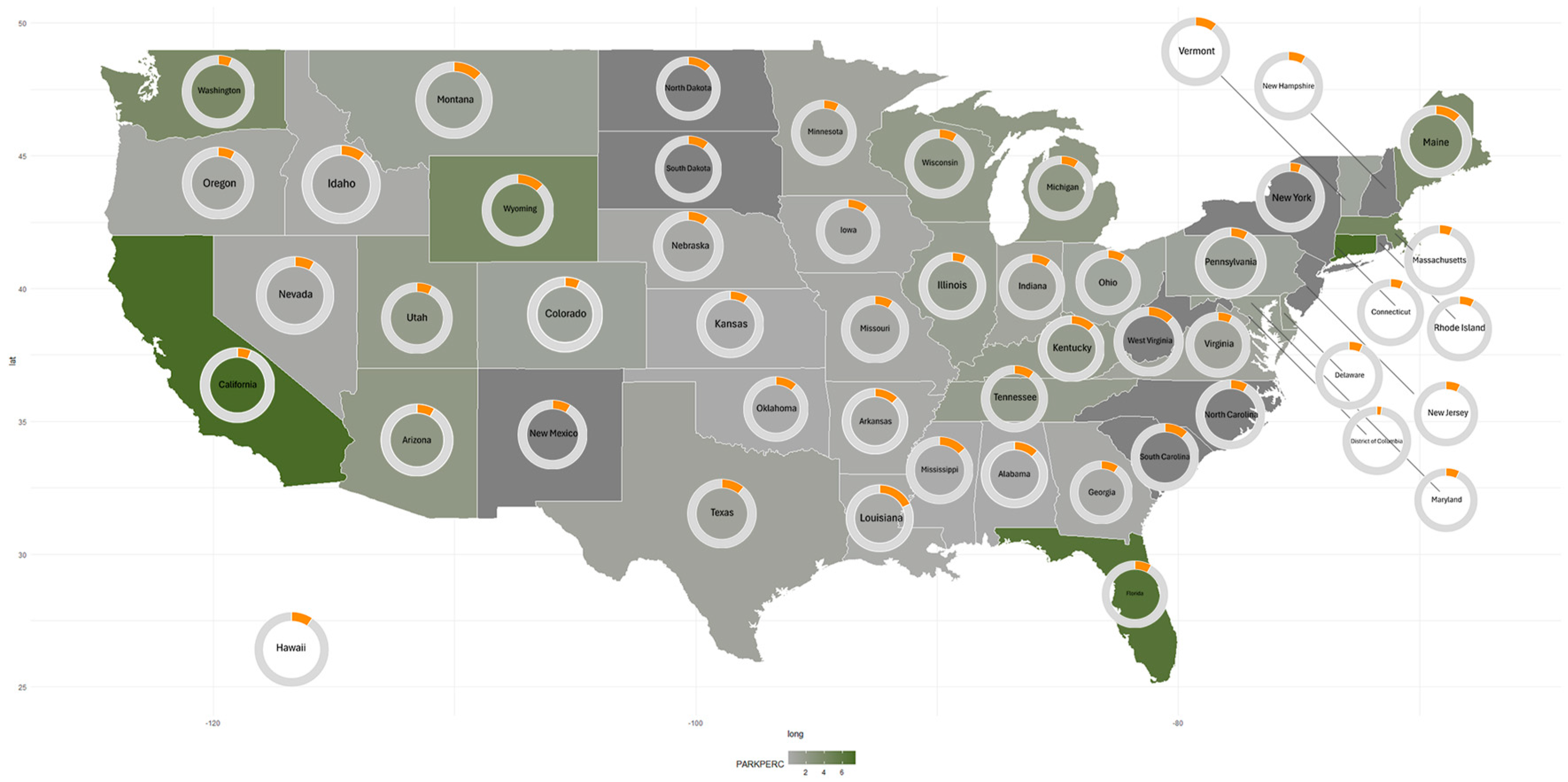
Biodiversity area density and energy density in the United States. Note: the greener the state is, the more biodiverse (higher nature park percentage of the total area) the state is. In circles, a share of energy expenditures of total state GDP is depicted. Source: author’s work based on Khan et al. [9,10].
Biodiversity area density and energy density in the United States. Note: the greener the state is, the more biodiverse (higher nature park percentage of the total area) the state is. In circles, a share of energy expenditures of total state GDP is depicted. Source: author’s work based on Khan et al. [9,10].
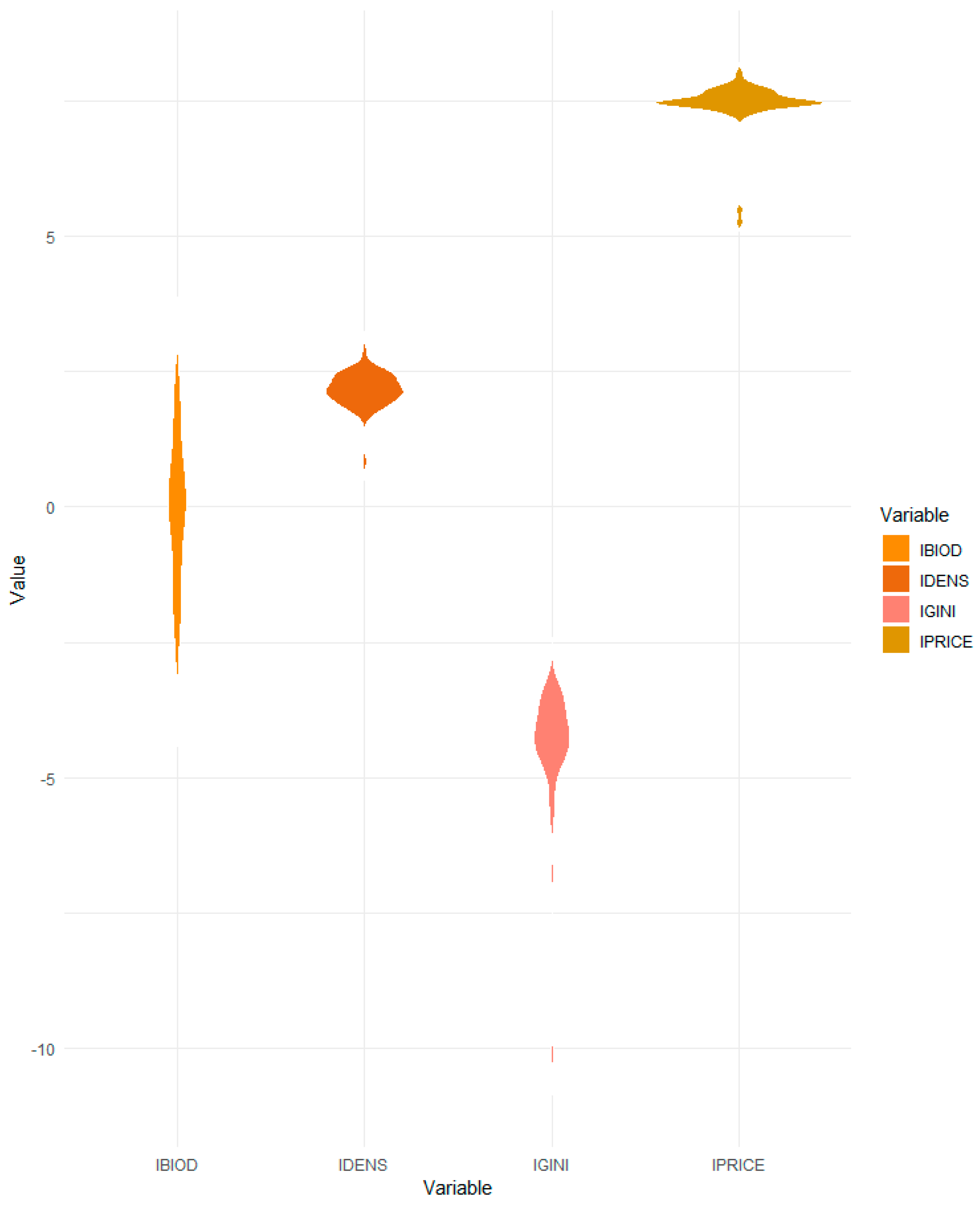
Distributions for variables in estimation.
Figure 3.
Distributions for variables in estimation.
Correlation matrix for variables in estimation.
Figure 4.
Correlation matrix for variables in estimation.

Results visualized. Notes: ** and * denote statistically significant at 5% and 10%, respectively.
Figure 5.
Results visualized. Notes: ** and * denote statistically significant at 5% and 10%, respectively.
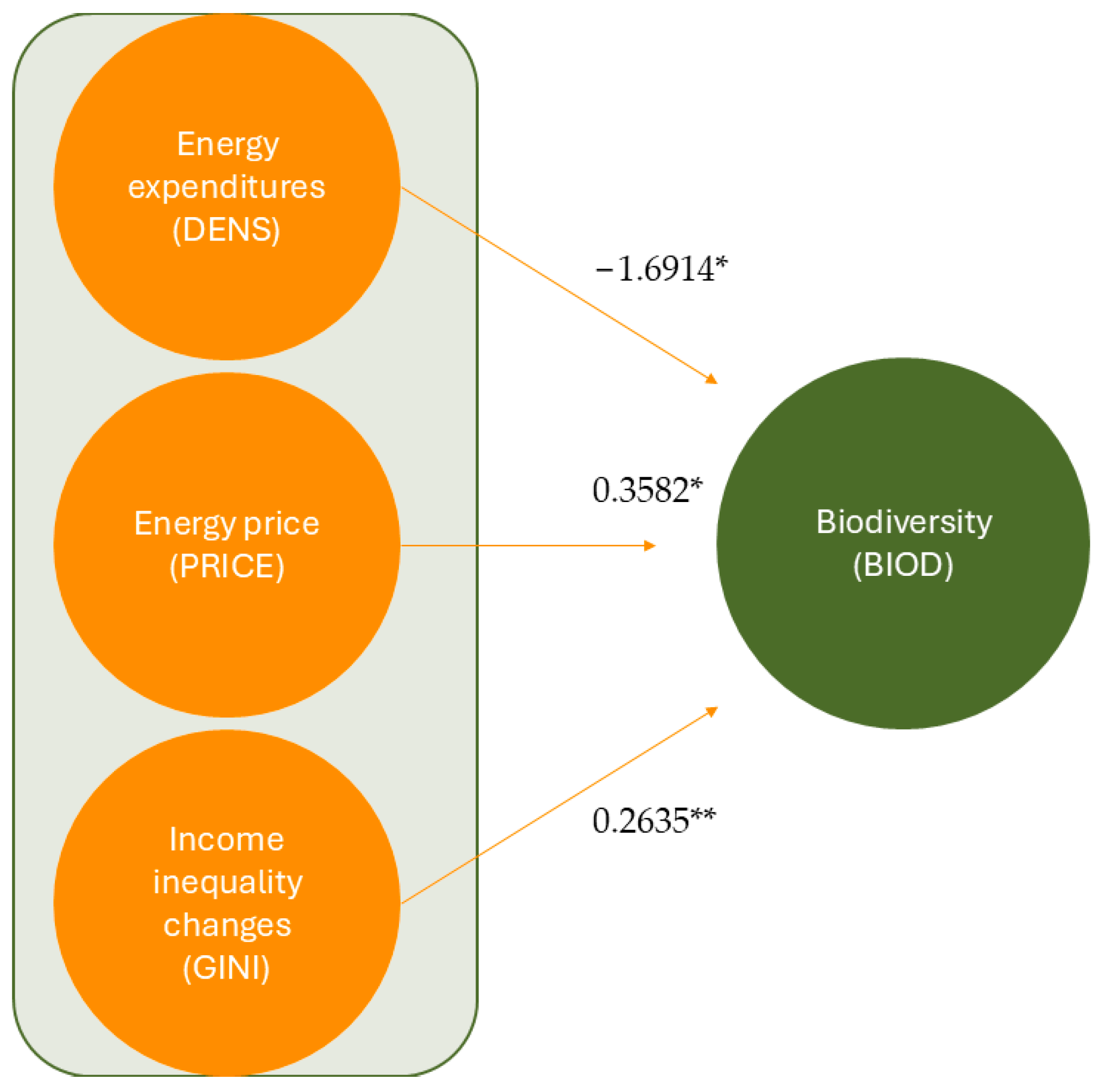
Table 1.
Data sources.
| Variable | Full Name of the Variable | Units | Source |
|---|---|---|---|
| BIOD | Nature park area percentage from the total area of the state | Per cent | [9] |
| DENS | Energy expenditures as a per cent of current-dollar GDP | Per cent | [10] |
| PRICE | Price of electricity consumed | Dollars per Million Btu | [10] |
| GINI | Change in the Gini index between 1990 and 2010 | Index | [23] |
Table 2.
Summary statistics.
Table 2.
Summary statistics.
| Variable | Obs. | Std. Dev. | Min | Max | Mean |
|---|---|---|---|---|---|
| BIOD | 50 | 1.3236 | −2.8134 | 2.2418 | −0.0823 |
| DENS | 51 | 0.3165 | 0.8502 | 2.8870 | 2.1706 |
| PRICE | 51 | 0.4533 | 5.2679 | 8.0311 | 7.4570 |
| GINI | 40 | 1.1686 | −10.1274 | −3.1814 | −4.4294 |
Table 3.
Estimation results for biodiversity.
Table 3.
Estimation results for biodiversity.
| Variable | Coefficient | Robust Std. Err. |
|---|---|---|
| DENS | −1.6914 * | 0.8372 |
| PRICE | 0.3582 * | 0.2046 |
| GINI | 0.2635 ** | 0.1059 |
| Const. | 2.1291 | 2.6457 |
| F | 8.39 | |
| Prob > F | 0.0002 | |
| R2 | 0.2991 | |
| Root MSE | 1.0433 |
Disclaimer/Publisher’s Note: The statements, opinions and data contained in all publications are solely those of the individual author(s) and contributor(s) and not of MDPI and/or the editor(s). MDPI and/or the editor(s) disclaim responsibility for any injury to people or property resulting from any ideas, methods, instructions or products referred to in the content. |
Source link
Anna Auza www.mdpi.com