Identifying Key Indicators for Successful Foreign Direct Investment through Asymmetric Optimization Using Machine Learning

Considering the literature review on improved solutions for determining the significance of FDI indicators, many of which are computer-based and often utilize machine learning (ML) techniques, it can be concluded that ensemble ML methods are currently a trend for solving such complex problems. However, the existing literature still lacks a sufficient number of references that integrate multiple ML methods, whether different or of the same type. This gap motivated the authors to conduct further research into such methods.

To evaluate the proposed model, the authors used datasets available on the World Bank’s website, which are detailed later in this section. For practical implementation, the dataset first required preprocessing, as described in a subsequent part of this paper. The preprocessed data were then analyzed, classifying all instances where the average FDI as a percentage of GDP was greater than 5% during the period from 2017 to 2021 into two categories: positive and negative (for values below 5%). This classification allowed the positive class to include countries where the conditions were favorable enough for the occurrence of successful FDI.

2.1. Methods

The problem under consideration, with the described dataset preprocessing, falls into the category of classification problems. Two main groups of methods are available for solving such problems: traditional statistical methods like logistic regression and feature selection.

In a logistic regression model, when the dependent variable takes on a finite set of values, the relationship between predictors—which can be continuous, binary, or categorical—and the dependent variable, which in this case is binary, is described. For binary outcomes, we implement binary regression, as is the case here. However, if the dependent variable has three or more categories, nominal logistic regression may be applied. Additionally, if the dependent variable has three or more categories that can be ranked, though the distances between them are not necessarily equal, ordinal logistic regression is appropriate. One might question whether linear regression can still be used in classification problems. The dependent variable is treated as a Bernoulli random variable, denoted as BinaryVariable in Equation (1) in the case of binary regression, where the two categories are coded as 0 or “false” for failure and 1 or “true” for success.

$B i n a r y V a r i a b l e = \begin{matrix} 0 (f a l s e) - failure \\ 1 (t r u e) - s u c c e s s \end{matrix}$

(1)

Since the dependent variable follows a Bernoulli distribution rather than being a continuous random variable, the errors cannot be normally distributed. Additionally, applying linear regression would result in nonsensical fitted values, possibly falling outside the 0, 1 range. In cases involving a binary dependent variable, one potential approach is to classify a “success” if the predicted value exceeds 0.5 and a “failure” if it does not. This method is somewhat comparable to linear discriminant analysis, which will be discussed later. However, this technique only produces binary classification results. When the predicted values are near 0.5, the confidence in the classification decreases. Furthermore, if the dependent variable contains more than two categories, this method becomes unsuitable, requiring the use of linear discriminant analysis instead.

Machine learning (ML) is a broad discipline grounded in statistical analysis and artificial intelligence, focused on acquiring knowledge, such as learning rules, concepts, and models that should be interpretable and accepted by humans. In the ML process, it is essential to validate the knowledge acquired, meaning the learned rules, concepts, or models must undergo evaluation. Two main evaluation methods exist, both involving the division of the available dataset into learning and testing sets in different ways.

The first method is the holdout test suite, where the dataset is split into two non-overlapping subsets: one for training and the other for testing the classifier (e.g., a 70:30 ratio). The classification model is built using the training data, and its performance is evaluated using the test data, allowing an assessment of classification accuracy based on the test results.

The second method, K-fold cross-validation, is more effective than using a single test set. In this approach, the dataset is split into k equal parts (or folds). One fold is used for testing, while the remaining folds are used for training. Predictions are made based on the current fold, and the process is repeated for k iterations, ensuring each fold is used for testing exactly once. The accuracy of the learned knowledge is one key measure of success, defined as the ratio of successful classifications to the total number of classifications. Other common evaluation metrics include precision, recall, the F1 measure, and, importantly, the Receiver Operating Characteristic (ROC) curve. Additionally, when dealing with imbalanced datasets, the precision–recall curve (PRC) may be more relevant, as will be discussed later in this chapter.

An important fact that must be noted is that the variables choice in the classification process affects all performance metrics of classification. Therefore, different techniques for variable selection are necessary during the data preparation or preprocessing phase, and dimension reduction methods may also be applied.

This paper proposes an ensemble ML model for determining the significance of various FDI indicators and predicting the likelihood of successful FDI in a given country based on these factors. As mentioned earlier, the proposed method integrates several feature selection algorithms, a binary regression algorithm, and the best-performing classification algorithm, combining them into a stacking ensemble ML method. The following subsections will briefly describe the methodologies employed, as the ensemble method integrates logistic binary regression with ML-based classification methods and feature selection techniques.

2.1.1. Classification Methodology

Classification algorithms are part of supervised machine learning (ML) and are commonly used for predictive modeling tasks. In the novel model proposed in this paper, these algorithms are utilized as the combiner in a stacking ensemble method. At the start of the procedure, the best algorithm is selected from several types across different groups, ideally choosing the best option from each group. The classification methodology relies on the existence of labeled instances in more than one class (or attribute) of objects, allowing it to classify the categorical class (attribute) value based on the remaining factors or attributes [41]. Selecting the appropriate classification algorithm for a specific application is not only the first step but also one of the most critical aspects of the ML process, which is especially important when such methodology is applied to large datasets. To address the problem considered in this paper, the proposed ensemble model uses a classification approach that categorizes instances into two classes: positive or negative, corresponding to “true” or “false”. The possible outcomes of this classification are displayed in the confusion matrix, as shown in Table 1.

Let N denote the total number of members in the considered set, as shown in Table 1. This value is the sum of positive and negative cases, i.e., TP + FN + FP + TN = N, where TP represents true positives, FN false negatives, FP false positives, and TN true negatives. All results presented in Table 1, for the case of two-class classification, can be used to calculate the most important classification metrics—accuracy, precision, recall, and the F1 measure—using the following formulas:

$Accuracy = (TP + TN) / N \in [0, 1]$

(2)

$Precision = TP / (TP + FP) \in [0, 1]$

(3)

$Recall = TP / \in (TP + FN) \in [0, 1]$

(4)

$F 1 measure = 2 \cdot \frac{precision \cdot recall}{precision + recall} \in [0, 1]$

(5)

In evaluating the performance of any classifier, the Receiver Operating Characteristic (ROC) curve is commonly used as one of the most important measures. It represents the false positive rate on the OX axis and the true positive rate on the OY axis [42]. For instance, point (0, 1) signifies perfect classification, where all samples are correctly classified, while point (1, 0) indicates a classification where all samples are incorrectly classified. The output in ROC space generated by naive neural networks or Bayes classification algorithms is a score—a numeric value that represents probability—whereas discrete classifiers yield a single point. In both cases, they express the likelihood that a particular instance belongs to a specific class [43]. The area under the curve (AUC) is a commonly used metric for measuring the accuracy of a model, with AUC values greater than 50% considered acceptable and values above 70% indicating good classification performance.

For imbalanced datasets, however, the precision–recall curve (PRC) is a more suitable measure than the ROC AUC [44]. Similar to the ROC curve, PRC plots are generated by connecting pairs of precision and recall values at each threshold. A good classifier will have a PRC that approaches the upper-right corner. In general, the closer a point is to the position where both precision and recall are 100%, the better the model’s performance. Like with ROC, the area under the precision–recall curve (AUPRC) is a reasonable measure of performance, with AUPRC > 0.5 indicating acceptable performance and higher values reflecting better classifier performance.

In practical terms, classification is a machine learning task but can also be considered a data mining task involving the separation of instances in a dataset into one of the predetermined classes based on the values of input variables [45]. The literature review shows that the most commonly applied classifiers include Bayes networks, decision trees, neural networks, and K-Nearest Neighbor, among others. For the proposed model, it is essential to use at least five of the most popular classification algorithms. The authors selected algorithms from different groups as categorized in WEKA software, version 3.8.6 [46], including types from Bayes, Meta, Trees, Misc, Rules, Lazy, and Functions. Below, a brief description of a selected algorithm from each of these groups is provided.

The Naive Bayes classifier [47] is one of the oldest classification algorithms and generates a model based on Bayes’ theorem. The term “naive” refers to the simplifying assumption it makes: the factors used in classification are conditionally independent, and there are no hidden factors that could influence the classification. These assumptions allow the Naive Bayes classifier to perform classification efficiently. For conditionally independent factors A1, A2, …, Ak, the probability of the class factor A is calculated using the following rule:

$P (A_{1}, \dots, A_{k} | A) = \prod_{i = 1}^{k} (A_{i} | A)$

(6)

The main advantage of this classifier is the convenience of small datasets.

Bagging, or Bootstrap Aggregating, is an ensemble method from the Meta group of classifiers that enhances the stability and accuracy of weak estimators or classification models. Breiman [48] introduced Bagging as a technique for reducing variance in a given base model, such as decision trees or other methods that involve selecting variables and fitting them into a linear model. Random forest [49] belongs to the Trees group of commonly used classifiers. Tree-structured classifiers are an attractive choice for solving one classification or prediction problem because they are easy to interpret.

The PART classifier [50] from the Rules group in Weka builds partial decision trees. Each iteration utilizes the C4.5 decision tree algorithm to generate the best leaf and derive a corresponding rule for the tree. This approach is particularly useful in binary classification, as applied in this paper.

SMO [51], from the Functions group in Weka, is an efficient optimization algorithm used in the implementation of support vector machines (SVMs). Although it is not one of the most commonly used classifiers, it is applied in this paper due to its suitability for binary classification with both numerical and binary factors, which aligns with the problem being addressed.

InputMappedClassifier belongs to the Misc group of Weka, but the IBk classifier belongs to the Lazy group, and both of them are not oft-used classifiers, and that is why we will not waste space describing them in more detail [52].

2.1.2. Logistic Regression

In logistic regression, when solving a problem using machine learning (ML) methodology, it is important to use probabilistic classifiers that not only return the label for the most likely class but also provide the probability of that class. These probabilistic classifiers can be evaluated using a calibration plot, which shows how well the classifier performs on a given dataset with known outcomes—this is especially relevant for the binary classifiers considered in this paper. For multi-class classifiers, separate calibration plots are required for each class.

In the proposed model, the authors applied the basic idea of univariate calibration, where logistic regression transforms classifier scores into probabilities of class membership in a two-class scenario. Many other authors have extended this concept to multi-class cases, as in [53].

The primary objective of logistic regression is to produce the best-fitting model that explains the relationship between a dichotomous dependent variable (the characteristic of interest) and a set of independent variables. Logistic regression generates coefficients in a formula that predicts or classifies a logit transformation of the probability of the characteristic’s presence, often denoted as p (including the standard error and significance level). This is defined as the logged odds, represented by logit(p):

$l o g i t (p) = b_{0} + b_{1} X_{1} + b_{2} X_{2} + \dots + b_{k} X_{k}$

(7)

$o d d s = \frac{p}{1 - p} = \frac{probability of characteristics presence}{probability of characteristics absence}$

(8)

$l o g i t (p) = l n (\frac{p}{1 - p})$

(9)

The coefficients in the logistic regression equation are represented by b₀ b₁, b₂, …, b_k. These coefficients indicate whether the corresponding independent variables have an increasing or decreasing effect on the dependent variable, with b_i > 0 indicating an increasing effect and b_i < 0 indicating a decreasing effect. When the independent variables are dichotomous, their impact on the dependent variable can be determined by simply comparing their regression coefficients. By exponentiation of both sides of the regression equation (as shown in Equations (7) and (9)), the equation can be transformed into a well-known form of logistic regression:

$o d d s = \frac{p}{1 - p} = e^{b_{0}} \cdot e^{b_{1} X_{1}} \cdot e^{b_{2} X_{2}} \cdot e^{b_{s} X_{s}} \cdot \dots \cdot e^{b_{k} X_{k}}$

(10)

As is evident from the provided Formula (10), when variable Xi increases by 1 unit and all other parameters remain unchanged, then the odds will increase by a value of parameter e^b_i.

$e^{b_{t} (1 + X_{t})} - e^{b_{t} X_{t}} = e^{b_{t} X_{t}} = e^{b_{t} (1 + X_{t}) - b_{t} X_{t}} = e^{b_{t} + b_{t} X_{t} - b_{t} X_{t}} = e^{b_{t}}$

(11)

The factor e^b_i represents the odds ratio (O.R.) for the independent variable X_i.

It indicates the relative change in the odds of the outcome: when the O.R. is greater than 1, the odds increase, and when it is less than 1, the odds decrease. This change occurs when the value of the independent variable increases by one unit.

Logistic regression can be implemented using various statistical software programs, with SPSS [54] being one of the most commonly used tools. SPSS provides three basic methods for binary regression: the enter method, the stepwise method, and the hierarchical method. In this paper, the authors employed the standard enter method for the proposed model. In the hierarchical method, researchers determine the order in which independent variables are added to the model. Stepwise methods include two categories: forward selection and backward elimination. The basic characteristic of the enter method is that it includes all independent variables in the model simultaneously. All methods aim to remove independent variables that are weakly correlated with the dependent variable from the regression equation.

2.1.3. Future Selection Techniques

Machine learning classification methods are sensitive to data dimensionality, making it evident that applying various dimensionality reduction techniques can significantly improve results. Algorithms for feature subset selection perform a space search based on candidate evaluation [55]. Several evaluation measures have proven effective in removing irrelevant and redundant features, including the consistency and the correlation measures. The consistency measure seeks to identify the minimum number of features that consistently differentiate class labels, defining inconsistency as instances where two cases have different class labels but share the same feature values.

The most common taxonomy for feature selection methods divides them into three groups [56]:

Filter: Known examples include Relief, GainRatio, and InfoGain;
Wrapper: Notable examples include BestFirst, GeneticSearch, and RankSearch;
Embedded: These methods combine filter and wrapper techniques.

Weka, a widely used, free-to-use software, includes a feature selection function that reduces the number of attributes by applying different algorithms. This made it the tool of choice for evaluating the proposed model in the case study representing the problem discussed in this paper.

Since the first group of filter-based feature selection methods was used in the proposed model, the algorithms from this group are briefly described below. For a dataset denoted as S, the filter algorithm begins by creating an initial subset D1, which could be an empty set, the entire set, or a randomly selected subset. It then explores the feature space based on a predetermined search strategy. Each subset Di generated during the search is evaluated using an independent metric and compared to the current best subset. If it performs better, it becomes the new best subset. The search continues until a predefined stopping condition is met. The final output of the algorithm is the last best subset, which is considered the final result. The feature selection process often relies on entropy as a metric for assessing the purity of a set of examples, considering the measure of unpredictability in the system. The entropy of Y is as follows:

$H (Y) = - \sum_{y \subset Y} p (y) \cdot \log_{2} (p (y))$

(12)

Feature selection methods vary in how they handle the issues of irrelevant and redundant attributes. In the proposed model, the authors utilized multiple filter algorithms, more than the recommended minimum of five, covering all the filter algorithms available in the WEKA 3.8.6 software. All these algorithms were used with the Ranker search method, which produces a ranked list of attributes based on their individual evaluations. This method must be paired with a single-attribute evaluator, not an attribute-subset evaluator. In addition to ranking attributes, Ranker also selects them by eliminating those with lower rankings.

Considering that entropy can serve as a criterion for impurity in training set S, there is a way to define a measure that reflects the additional information each attribute provides, as determined by the class. This measure, known as information gain, represents the amount by which the entropy of the attribute is reduced. It is denoted as InfoGain and is used to evaluate the value of an attribute in relation to the class, calculated using the following formula:

$I n f o G a i n (C l a s s, A t t r i b u t e) = H (C l a s s) - H (C l a s s | A t t r i b u t e)$

(13)

where H represents the entropy of information, and the information gained about an attribute after observing the class is equal to the information gained when the observation is reversed.

The information gain ratio, referred to as GainRatio, is an asymmetrical measure that corrects the bias inherent in the InfoGain measure. It is essentially a modified version of InfoGain, designed to reduce its bias toward certain attributes, and is calculated using the following formula:

$G a i n R a t i o = \frac{I n f o G a i n}{H (C l a s s)}$

(14)

As shown in Formula (13), when predicting a specific variable or attribute, InfoGain is normalized by dividing it by the entropy of the class and vice versa. This normalization ensures that the GainRatio values fall within the range [0, 1]. A GainRatio of 1 means that knowledge of the class perfectly predicts the variable or attribute, while a GainRatio of 0 indicates no relationship between the variable or attribute and the class.

FilteredAttributeEval (ClassifierAttributeEval) is a classifier that handles nominal and binary classifications with various types of attributes, including nominal, string, relational, binary, unary, and even missing values. It uses an arbitrary evaluator on data processed through a filter built solely from the training data.

SymmetricalUncertAttributeEval, described in Equation (15), is a classifier that evaluates the significance of an attribute by calculating its symmetrical uncertainty, considering the presence of each class in the process.

$S y m m U (C l a s s, A t t r i b u t e) = 2 * (H (C l a s s) - H (C l a s s | A t t r i b u t e)) / H (C l a s s) + H (A t t r i b u t e)$

(15)

This classifier handles nominal, binary, and missing class classifications using attributes such as nominal, binary, unary, and others.

ReliefFAttributeEval is an instance-based classifier that randomly samples instances and examines neighboring instances from both the same and different classes, handling both discrete and continuous class data.

PrincipalComponents transforms the attribute set by ranking the new attributes according to their eigenvalues. A subset of attributes can optionally be selected by choosing enough eigenvectors to represent a specified portion of the variance, with the default set to 95%.

CorrelationAttributeEval evaluates the importance of an attribute by measuring its correlation (Pearson’s) with the class. For nominal attributes, each value is treated as an indicator and considered on a value-by-value basis. The overall correlation for a nominal attribute is calculated as a weighted average.

2.1.4. Ensemble Methods ML

As mentioned earlier in the Introduction and at the start of this section, ensemble methods are based on the concept that combining algorithms of different types can yield better results than each algorithm individually. There are several types of ensemble methods and their taxonomies, with the most commonly used being the following:

The following is a summary, as found in the literature [57]:

Ensemble learning combines multiple machine learning algorithms into a single model to enhance performance. Bagging primarily aims to reduce variance, boosting focuses on reducing bias, and stacking seeks to improve prediction accuracy;
While ensemble methods generally offer better classification and prediction results, they require more computational resources than evaluating a single model within the ensemble. Thus, ensemble learning can be seen as compensating for less effective learning algorithms by performing additional computations. However, it is important to note that in many problems, including the case study presented in this paper, real-time computation is not a constraint, making this extra computational effort manageable.

Stacking

The stacking ensemble algorithm involves training multiple machine learning algorithms and combining their predictions or classifications into a single model. This approach typically yields better performance than any individual algorithm alone [58]. Stacking can be applied to both supervised learning tasks and unsupervised learning tasks. In stacking, each algorithm is trained using the available data, and then a meta-algorithm is trained to make the final estimation, classification, or prediction. This process often involves cross-validation to prevent overfitting [59]. While logistic regression is commonly used as the combiner algorithm in practice, the proposed model in this article uses feature selection algorithms for this role.

2.1.5. Proposed Ensemble Model

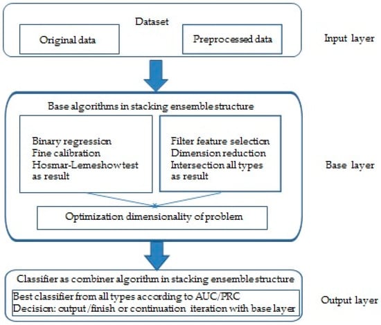
The authors acknowledge the potential negative effects of poor model fit in regression and the impact of imbalanced data in feature selection and classification, which has been noted in the prior literature [60,61]. As a result, they question the reliance on regression or feature selection combined with classification as the primary methods for solving binary classification problems, such as the one they are addressing in this paper. Therefore, as mentioned in the Introduction, the authors chose to apply a stacking methodology that incorporates both binary regression and feature selection methods, with a suitable classification algorithm serving as the combiner in the proposed model.

The proposed stacking ensemble method integrates two types of machine learning algorithms in an asymmetric structure. The first is a binary regression method that initiates the model and evaluates the goodness of fit at each step, while the second is a feature selection algorithm that reduces the dimensionality of the problem by selecting fewer factors. This process continues as long as the classification algorithm, acting as the combiner, permits it. The combiner only grants permission if the dimensionally reduced problem yields better values in terms of PRC (for imbalanced datasets) or ROC AUC (for balanced datasets) before the iterative process begins.

The goodness of the regression model is assessed using the Hosmer–Lemeshow test, and ultimately, the significance coefficients of the final regression model with acceptable fit will refine the prediction by identifying the most important factors.

In this way, the authors aim to develop an optimized iterative procedure that combines the strengths of both methods while minimizing their weaknesses. Although both binary regression and feature selection algorithms are widely recognized as supervised learning techniques used for predictions on labeled datasets, their divergent approaches to binary classification and other machine learning problems highlight their differences.

The proposed model is provided with the algorithm presented in Figure 2 and described in Algorithm 1.

Algorithm 1: Determining the importance of indicators for successful FDI

1. * Input data each instace with n1 factors for m instances-countries and preprocess the data.
NEXT
Perform binary regression and determine

n \leq n 1

non-colinear input indicators;
Check regressions goodness

H L s i g \geq 0.05

IF NO No valid prediction GOTO END
ELSE
NEXT
Check datasets imbalance OneClass is <=25%ofOtherClass
IF NO No Treshold TR = ROC AUC
ELSE Treshold TR = PRC
NEXT
2. ** Perform classification with a minimum of five classification algorithms of different types and identify the algorithm ‘TheBest’ with the highest PRC (or ROC AUC) value.
Check goodness of classification

P R C | (R O C A U C) | \geq 0.7

IF NO No valid prediction GOTO END
ELSE
NEXT
3. *** Apply feature selection procedure using minimum 5 different filter algorithms; Using intrsection logic operation determine M <= N attributes;
NEXT
4. **** Using TheBest classification algorithm determine with dataset of M attributes new its value TheNewBest
NEXT
Check regressions goodness

H L s i g \geq 0.5

IF NO GOTO 6 ******
ELSE GOTO 5 *****
NEXT
5. **** Check goodness of classification

P R C | (R O C A U C) | \geq 0.7

IF NO GOTO 6 ******
ELSE GOTO 3 ***
NEXT
6. ****** By means of already carried out in the previous Step 5 binary regression determine important indicators for FDI i.e., prediction formula
END

* Step 1. Step 1 starts with an obligatory preprocessing dataset with n1 indicators and m instances—countries as independent variables. The last special column contains binary values of the dependent variable FDI in % of GDP, which indicates the success of FDI in each specific country. To be useful for the application preprocessed dataset, it must have a minimum of four instances, i.e., regions or countries for each used indicator of FDI and successful instances classified as true, each of which has an inflow of FDI in GDP greater or equal to five percent. Before entering the iterative loop, binary regression is made, and collinearity is checked to exclude potentially collinear indicators. The goodness of the Hosmer–Lemeshow model is tested, and if it is greater than 0.05, the procedure can start; otherwise, it is not applicable and cannot determine the significance of individual indicators. Also, before entering the procedure in Step 2, determination of the imbalance of the considered dataset is performed, and in the case of imbalance, i.e., if one of the two classes in the considered binary classification is present with less than 25% in the classification procedure, the PRC evaluator is used as the most significant in the selection of the best from a minimum of 5 different types of classification algorithms; otherwise, the ROC measure is used.

** Step 2. This step involves selecting the best classification algorithm for the model from at least five different types of classification algorithms. It concludes by evaluating the goodness of classification. If the value of the most significant measure, PRC (or ROC AUC), is less than 0.7, the procedure terminates, as it would not be applicable and cannot determine the significance of individual indicators. A 10-fold cross-validation test procedure is used.

*** Step 3. The loop itself begins with Step 3, in which a potential reduction in the dimensionality of the problem is determined between a minimum of five feature selection filter algorithms using a logical function of the intersection of individually obtained results, and the algorithm continues in Step 4.

**** Step 4. In Step 4, with a reduced number of indicators selected in Step 3 by the best classification algorithm, the PRC is determined by comparing an unbalanced set or ROC in the opposite case. It first examines the goodness of the regression model for that reduced number of indicators. If it is OK, it moves on to Step 5, and if there is no fulfillment of this condition, the procedure ends with a previously determined number of indicators in Step 6.

***** Step 5. In this step, it is checked whether the value of PRC, i.e., ROC, is now greater than or equal to the previous one. In the case of fulfillment of this condition, the loop continues with Step 3, and in the opposite case, the loop is exited in Step 6.

****** Step 6. If the optimization procedure for a specific dataset is possible, this algorithm ends with a previously determined number of indicators in Step 6, where significant indicators are determined based on the value of the regression model, and a prediction model can also be provided. The next step leads to the end of this algorithm.

2.2. Materials

The proposed model for estimating weight coefficients in this study is based on data and reports from the World Bank’s Enterprise Analysis Unit of the Development Economics Global Indicators Department [62]. However, the original datasets from the World Bank required preparation to be suitable for addressing the problem discussed in this paper. As a result, the data had to be preprocessed for use in the first step of the proposed model.

2.2.1. Dataset World Bank for FDI Countries around the World

The World Bank Enterprise Surveys (WBESs), part of the World Bank Enterprise Analysis Unit within the Development Economics Global Indicators Department, offer a vast array of economic data covering over 219,000 firms across 159 economies, with the expectation of reaching 180 economies soon. These surveys provide valuable insights into various aspects of the business environment, such as firm performance, access to finance, infrastructure, and more. The data are publicly available and are particularly useful for scientists, researchers, policymakers, and others. The data portal offers access to over 350 WBESs, 12 Informal Sector Enterprise Surveys in 38 cities, Micro-Enterprise Surveys, and other cross-economy databases.

The Enterprise Surveys focus on factors influencing the business environment, which can either support or hinder firms’ operations. A favorable business environment encourages firms to operate efficiently, fostering innovation and increased productivity, both of which are crucial for sustainable development. A more productive private sector leads to job creation and generates tax revenue essential for public investment in health, education, and other services. Conversely, a poor business environment presents obstacles that impede business activities, reducing a country’s potential for growth in terms of employment, production, and overall welfare.

These surveys, conducted by the World Bank and its partners, cover all geographic regions and include small, medium, and large firms. The surveys are administered to a representative sample of firms in the non-agricultural formal private economy. The survey universe, or population, is uniformly defined across all countries and includes the manufacturing, services, transportation, and construction sectors. However, sectors such as public utilities, government services, health care, and financial services are excluded. Since 2006, most Enterprise Surveys have been implemented under a global methodology that includes a uniform universe, uniform implementation methodology, and a core questionnaire.

The Enterprise Surveys collect a wide range of qualitative and quantitative data through face-to-face interviews with firm managers and owners, focusing on the business environment and firm productivity. The topics covered in the surveys are grouped into 13 categories, comprising over 100 indicators that impact FDI. These categories include firm characteristics, gender, workforce, performance, innovation and technology, infrastructure, trade, finance, crime, informality, regulations and taxes, corruption, and the biggest obstacles to doing business [63]. From the World Bank—Data Bank World Development Indicators [64], the authors have taken the data, which show what percent of FDI is in GDP for each country the authors include in this study.

2.2.2. Preprocessed Dataset World Bank for FDI 60 Countries around the World

The prepared and processed dataset that the authors used to evaluate the proposed model is provided as a Supplementary File for this paper. It is obtained on the following premises of the authors.

Keeping in mind the original data of the World Bank, the authors noticed the necessary reprocessing of the same in the next steps:

For more than a hundred indicators provided in 13 groups, a correct analysis would require about 500 instances, i.e., countries, and there are not that many in the world;
Data exist separately for companies of different sizes, but there are also aggregated data;
For individual countries, data for indicators as independent variables in the research are collected at intervals of about 5 years, and data for the dependent variable in the research for the percentage of FDI in the GDP of an individual country are available annually.

For these reasons, the authors, in the preprocessing of the dataset usable for the intended research, took data for a sufficient number of 60 countries that exist in the period of 5 years, 2017–2021. The independent variable included aggregate data for companies of all sizes and the average investment percentage in the same period for each of the countries included in the study. The dependent variable was shown to be successful in terms of FDI for the percentage of FDI greater than 5.

Source link

Aleksandar Kemiveš www.mdpi.com

Greenberg News

Identifying Key Indicators for Successful Foreign Direct Investment through Asymmetric Optimization Using Machine Learning

2.1. Methods

2.1.1. Classification Methodology

2.1.2. Logistic Regression

2.1.3. Future Selection Techniques

2.1.4. Ensemble Methods ML

2.1.5. Proposed Ensemble Model

2.2. Materials

2.2.1. Dataset World Bank for FDI Countries around the World

2.2.2. Preprocessed Dataset World Bank for FDI 60 Countries around the World

Greenberg

2.1. Methods

2.1.1. Classification Methodology

2.1.2. Logistic Regression

2.1.3. Future Selection Techniques

2.1.4. Ensemble Methods ML

2.1.5. Proposed Ensemble Model

2.2. Materials

2.2.1. Dataset World Bank for FDI Countries around the World

2.2.2. Preprocessed Dataset World Bank for FDI 60 Countries around the World

Related Posts

Greenpeace comment on the award of the Nobel Peace Prize to Nihon Hidankyo

Earth911 Inspiration: Fossil Free At Last

10 Sustainable Bamboo Clothing Options for Your Custom Wardrobe

Greenberg