Author Contributions
Conceptualization, K.B.T. and A.C.; Methodology, K.B.T.; Software, K.B.T.; Validation, K.B.T. and A.C.; Data curation, K.B.T. and A.C.; Writing—original draft, K.B.T.; Writing—review and editing, K.B.T. and A.C.; Visualization, K.B.T., A.C. and K.T.; Supervision, A.C. and K.T. All authors have read and agreed to the published version of the manuscript.
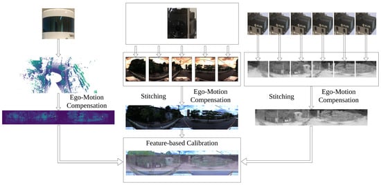
Visualization of the system including RGB cameras, thermal cameras, and LiDAR. 360 RGB camera and 360 thermal camera are made from independent cameras to remove blind spots. Images and point clouds are compensated to decrease negative impacts of motion. Then, point clouds and images are used for sensor calibration based on extracted features.
Figure 1.
Visualization of the system including RGB cameras, thermal cameras, and LiDAR. 360 RGB camera and 360 thermal camera are made from independent cameras to remove blind spots. Images and point clouds are compensated to decrease negative impacts of motion. Then, point clouds and images are used for sensor calibration based on extracted features.
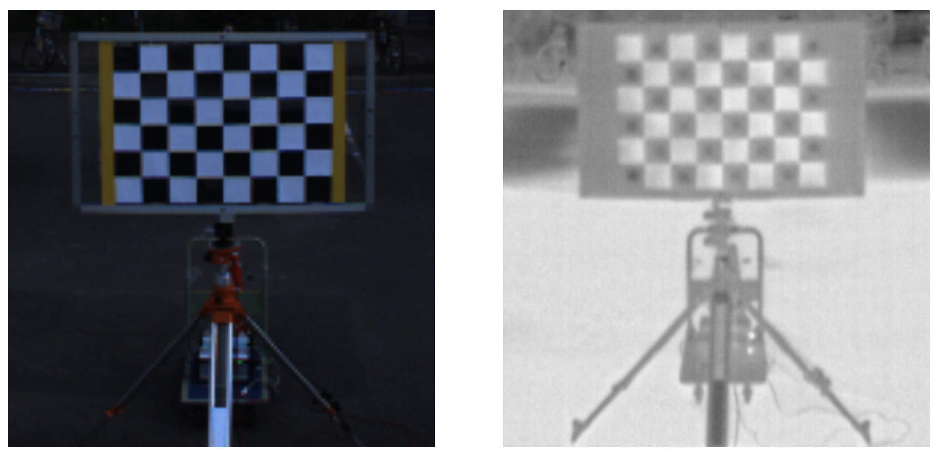
Visualization of the target detected by two types of cameras. The (left image) is the target detected by the RGB camera and the (right image) is the target detected by the thermal camera.
Figure 2.
Visualization of the target detected by two types of cameras. The (left image) is the target detected by the RGB camera and the (right image) is the target detected by the thermal camera.
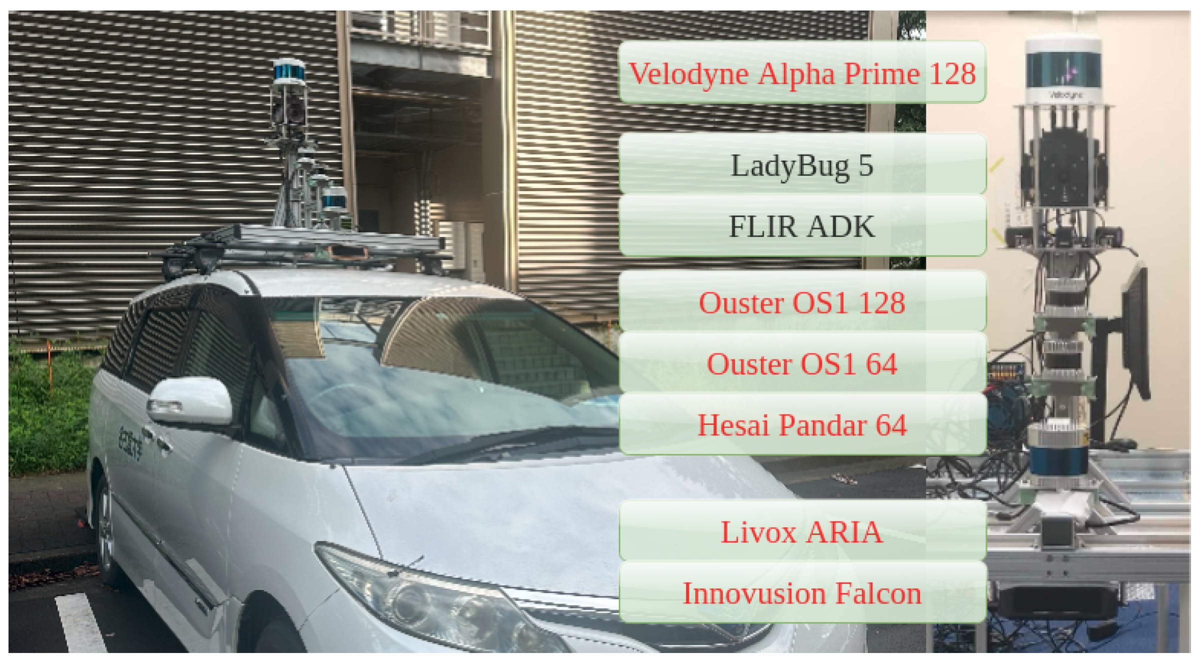
Our system includes sensors: LiDAR Velodyne Alpha Prime, LadyBug-5 camera, 6 FLIR ADK cameras, LiDAR Ouster-128, LiDAR Ouster-64 and LiDAR Hesai Pandar.
Figure 3.
Our system includes sensors: LiDAR Velodyne Alpha Prime, LadyBug-5 camera, 6 FLIR ADK cameras, LiDAR Ouster-128, LiDAR Ouster-64 and LiDAR Hesai Pandar.
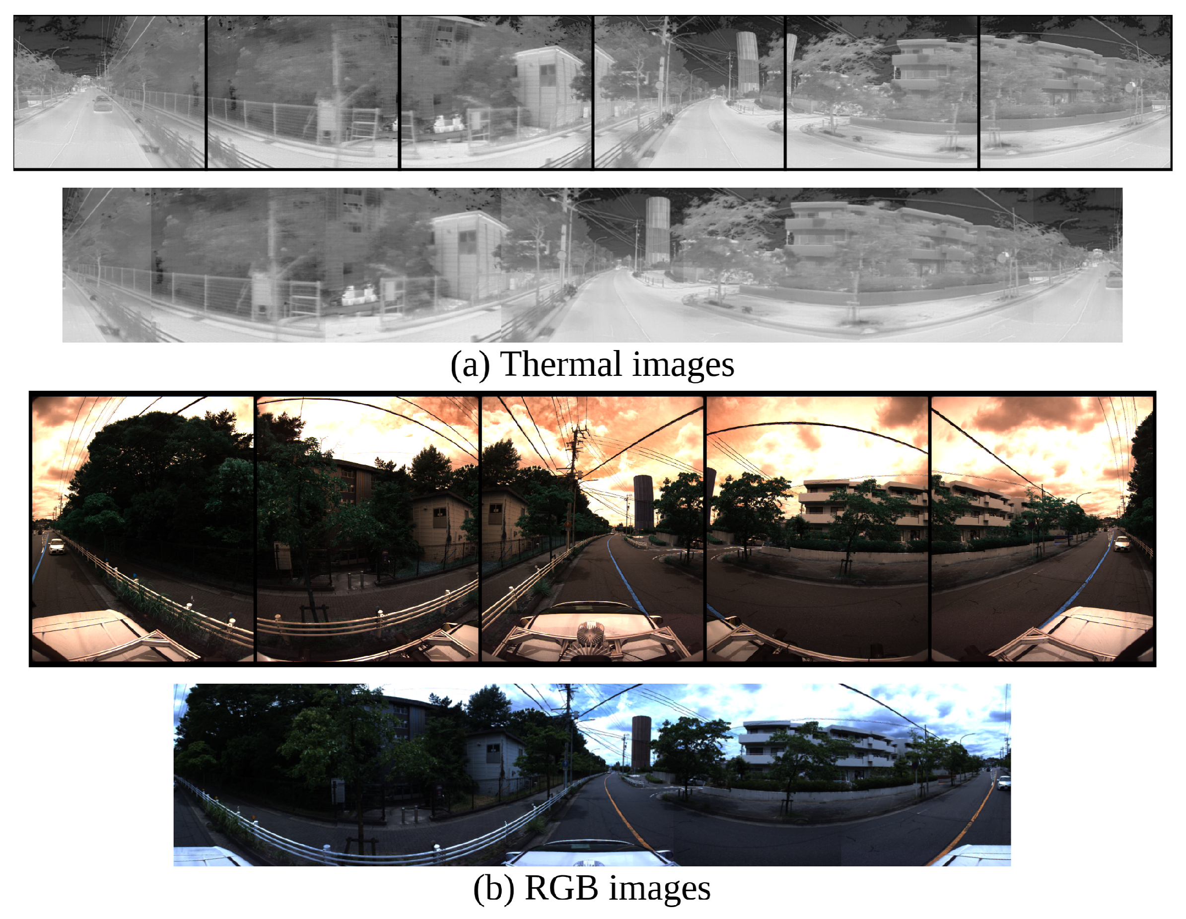
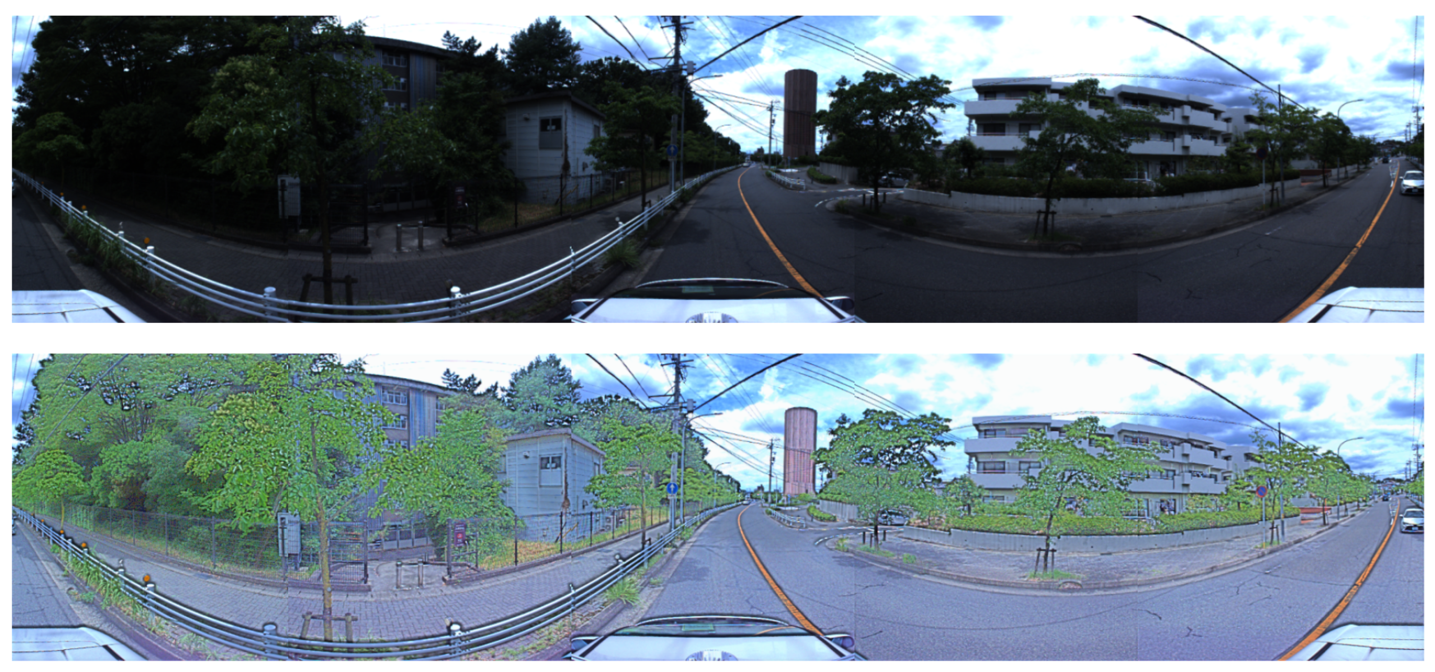
Visualization of stitching 360 thermal images and 360 RGB images.
Figure 4.
Visualization of stitching 360 thermal images and 360 RGB images.
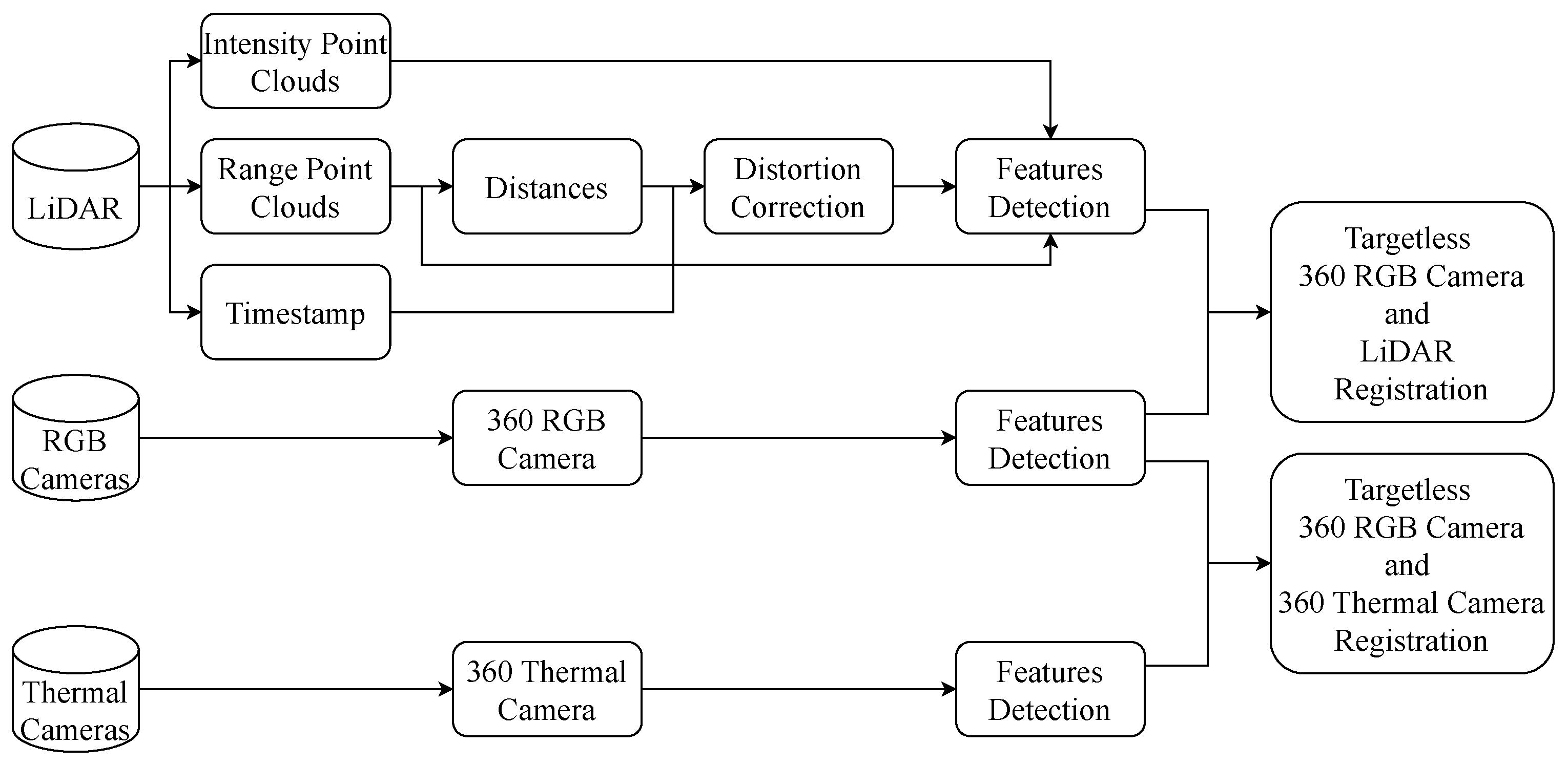
Pipeline of the registration process. The approach is divided into two parts, one part focuses on detecting key points from RGB images and thermal images, while the other part detects key points from images converted from LiDAR point clouds. For images generated from LiDAR point clouds, a velocity estimation step is required to perform distortion correction, ensuring the accurate positioning of the scanned points. After getting results from distortion correction, external parameters of LiDAR, 360 RGB camera and 360 thermal camera can be calibrated.
Figure 5.
Pipeline of the registration process. The approach is divided into two parts, one part focuses on detecting key points from RGB images and thermal images, while the other part detects key points from images converted from LiDAR point clouds. For images generated from LiDAR point clouds, a velocity estimation step is required to perform distortion correction, ensuring the accurate positioning of the scanned points. After getting results from distortion correction, external parameters of LiDAR, 360 RGB camera and 360 thermal camera can be calibrated.
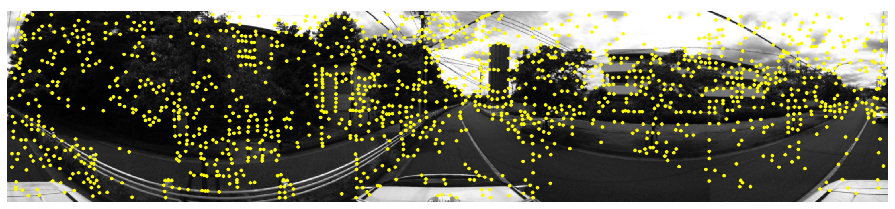
Visualization of features extracted from RGB images.
Figure 6.
Visualization of features extracted from RGB images.
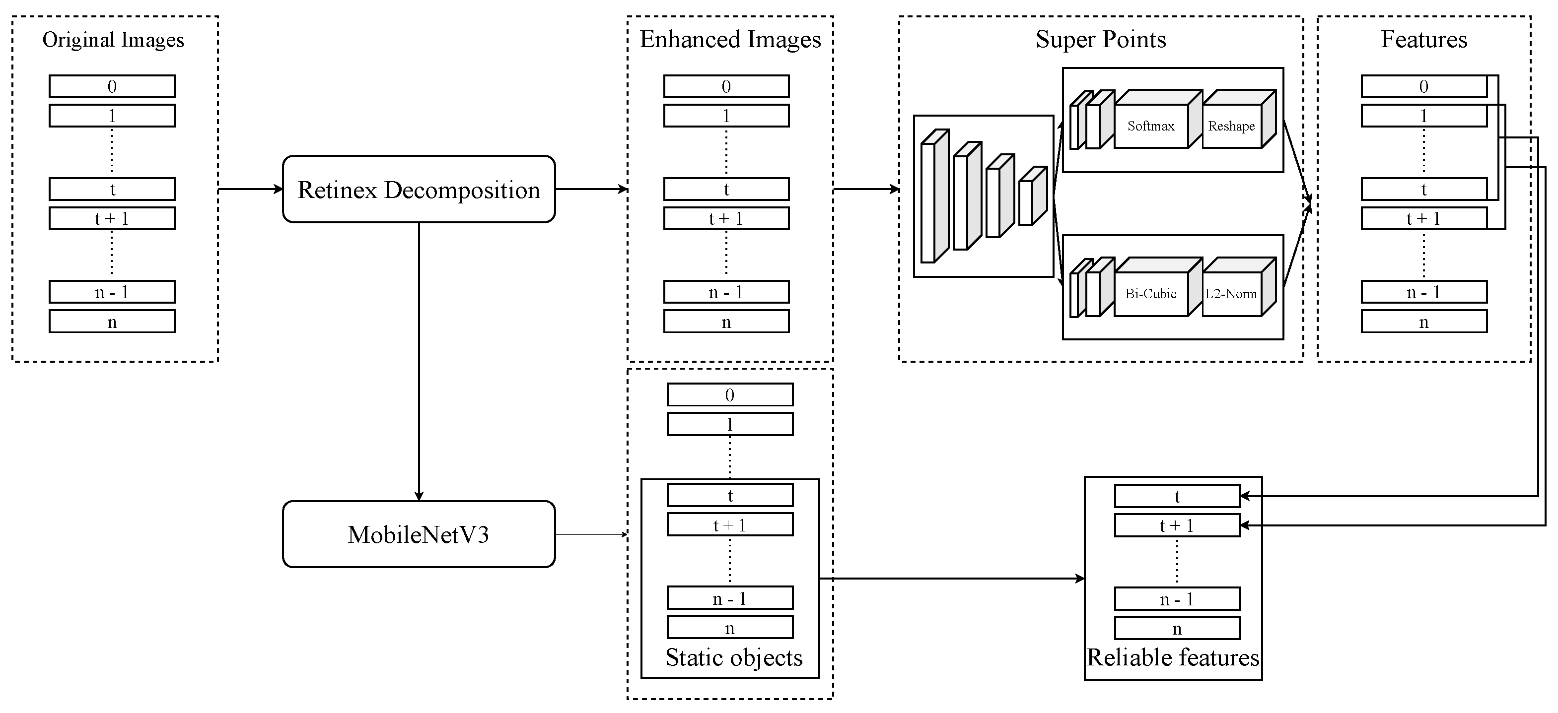
Pipeline of our approach. The first step is enhancing images by Retinex Decomposition. The second step is to extract key features from consecutive images. The third step is using MobileNetV3 to remove noise features on moving objects.
Figure 7.
Pipeline of our approach. The first step is enhancing images by Retinex Decomposition. The second step is to extract key features from consecutive images. The third step is using MobileNetV3 to remove noise features on moving objects.
The (above image) shows results before being enhanced by Retinex Decomposition. The (below image) shows results after being enhanced by Retinex Decomposition.
Figure 8.
The (above image) shows results before being enhanced by Retinex Decomposition. The (below image) shows results after being enhanced by Retinex Decomposition.
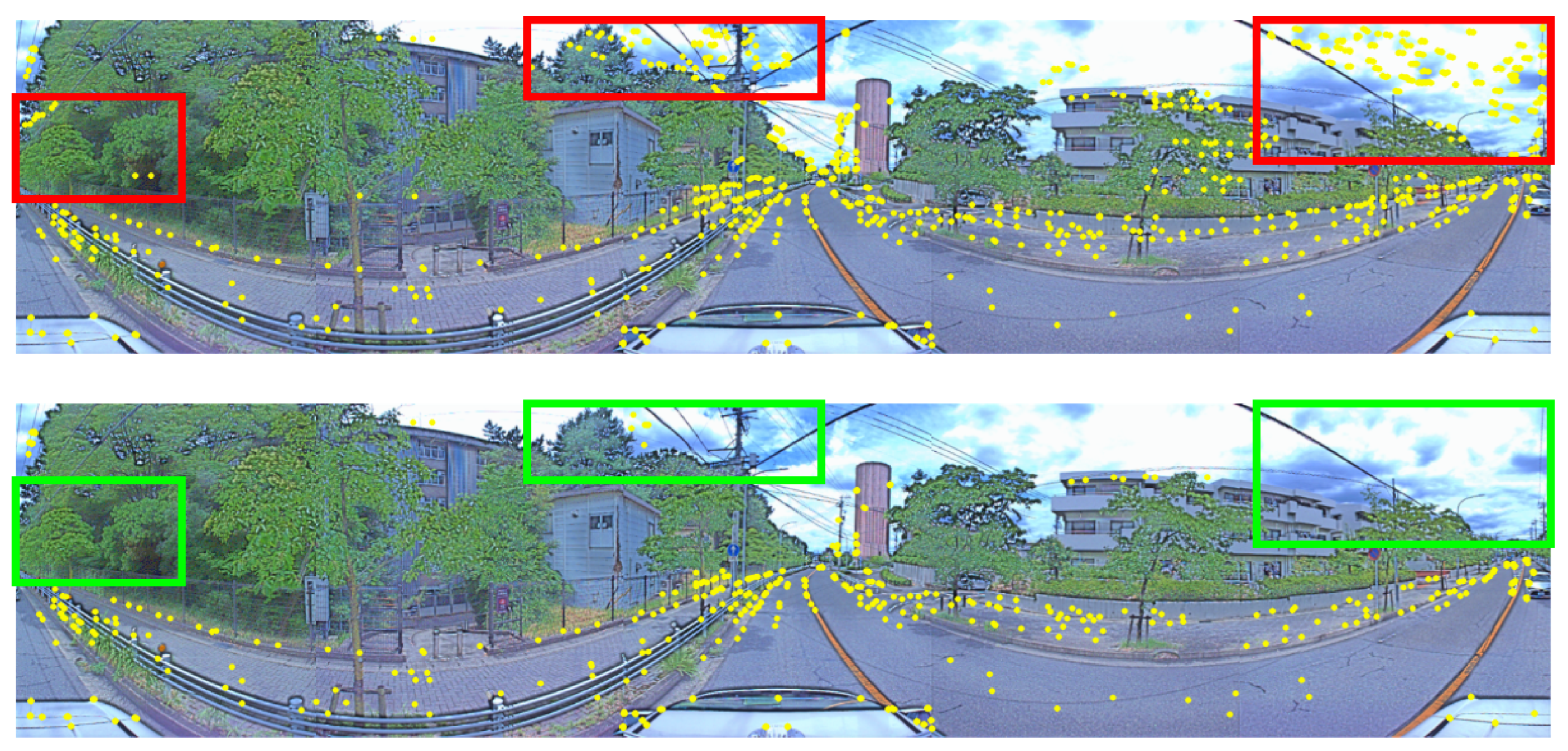
The (above image) including the red rectangles shows reliable features extracted from consecutive RGB images. The (below image) including the green rectangles shows reliable features after filtering by MobileNetV3.
Figure 9.
The (above image) including the red rectangles shows reliable features extracted from consecutive RGB images. The (below image) including the green rectangles shows reliable features after filtering by MobileNetV3.
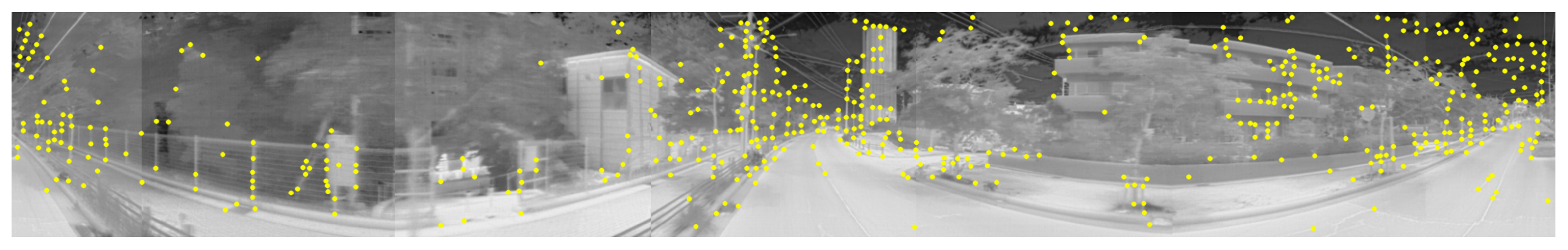
Visualization of features extracted from thermal images.
Figure 10.
Visualization of features extracted from thermal images.
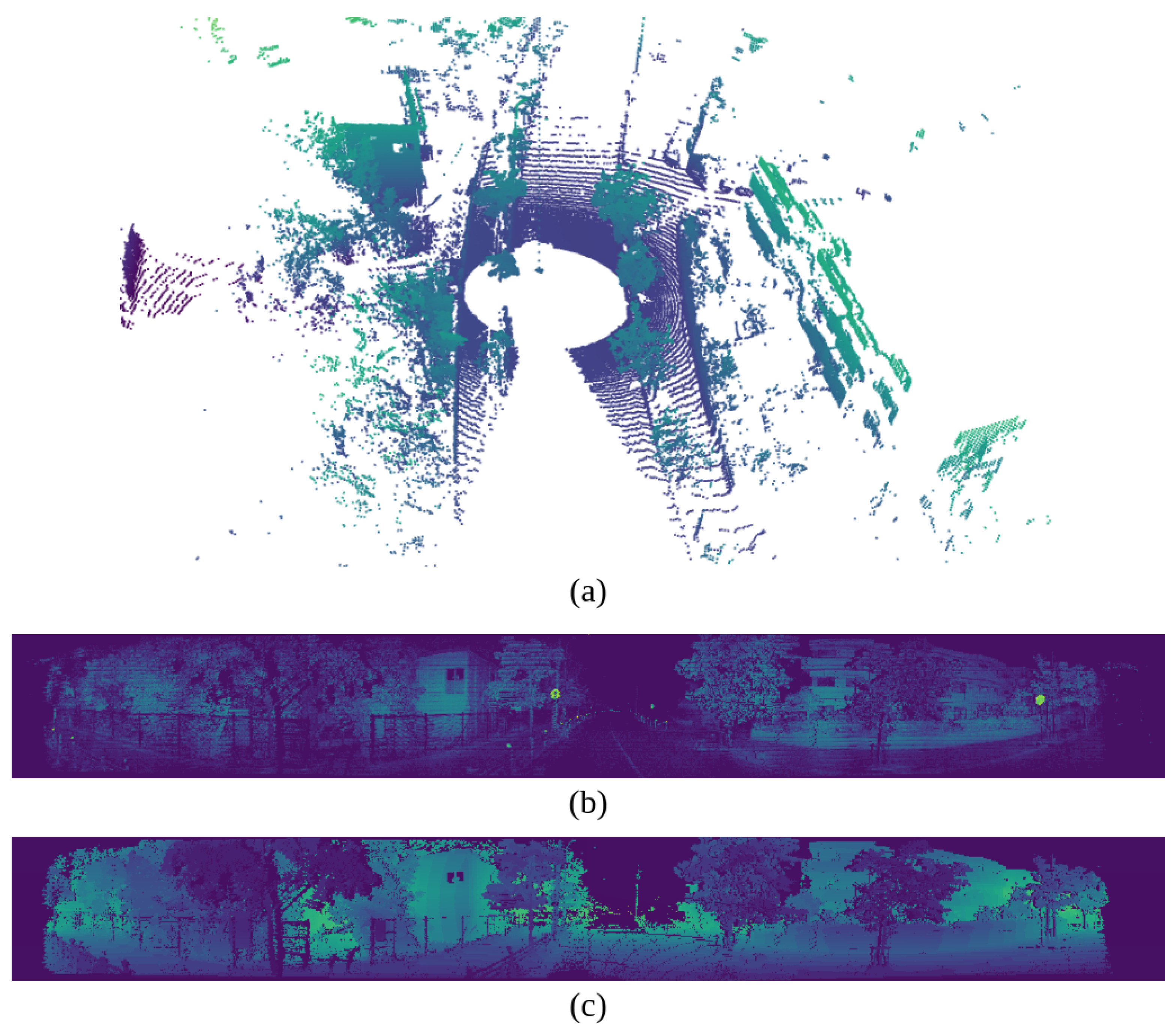
Visualization of image projection. (a) shows the 3D point cloud data from the LiDAR. (b) presents the 2D image data with the intensity channel. (c) presents the 2D image data with the range channel. The height of the image is 128, corresponding to the number of channels in the LiDAR.
Figure 11.
Visualization of image projection. (a) shows the 3D point cloud data from the LiDAR. (b) presents the 2D image data with the intensity channel. (c) presents the 2D image data with the range channel. The height of the image is 128, corresponding to the number of channels in the LiDAR.
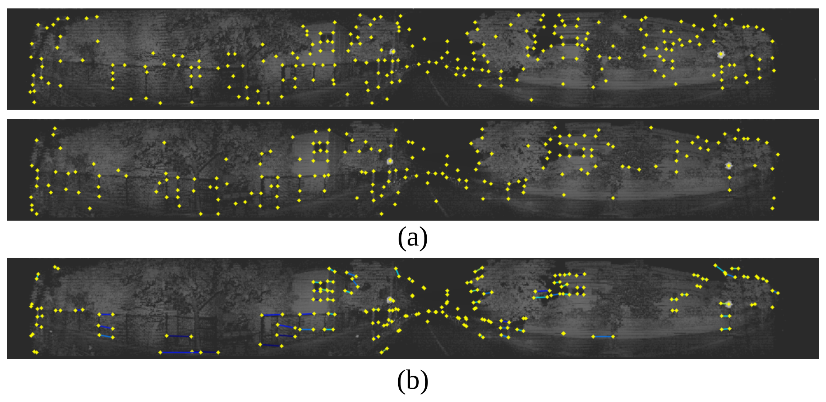
Visualization of key points extracted from LiDAR images. (a) simulates key points across two frames, while (b) simulates selecting key points with similarity across the two frames.
Figure 12.
Visualization of key points extracted from LiDAR images. (a) simulates key points across two frames, while (b) simulates selecting key points with similarity across the two frames.
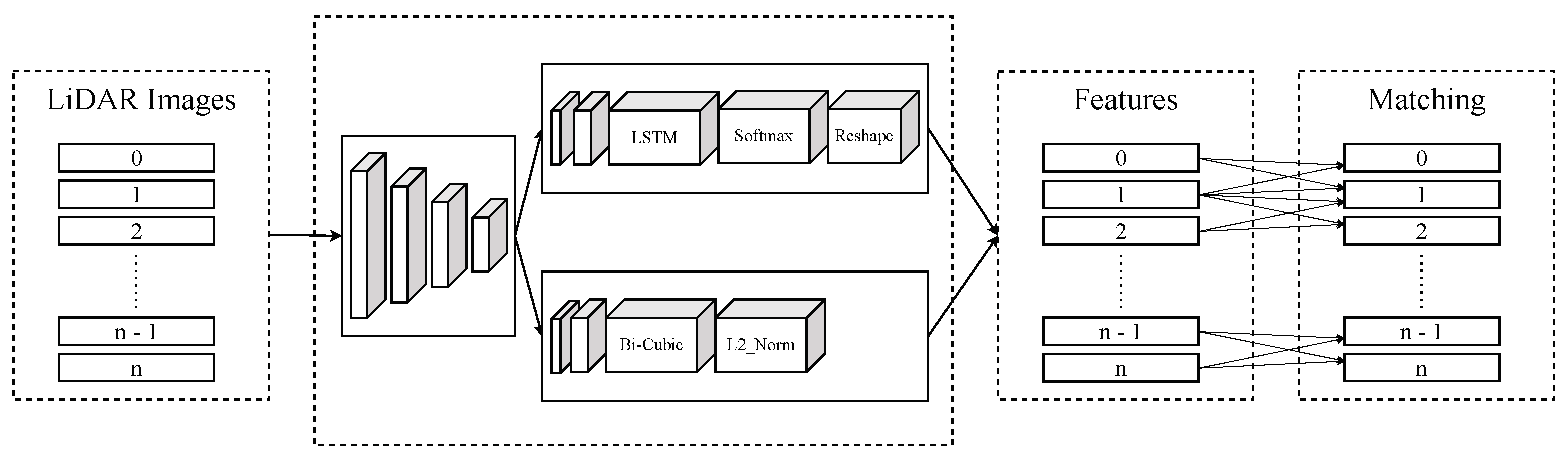
Pipeline of our approach. Key features of projected images are extracted by Superpoint enhanced by LSTM. These features are matched to find pair points in two consecutive frames.
Figure 13.
Pipeline of our approach. Key features of projected images are extracted by Superpoint enhanced by LSTM. These features are matched to find pair points in two consecutive frames.
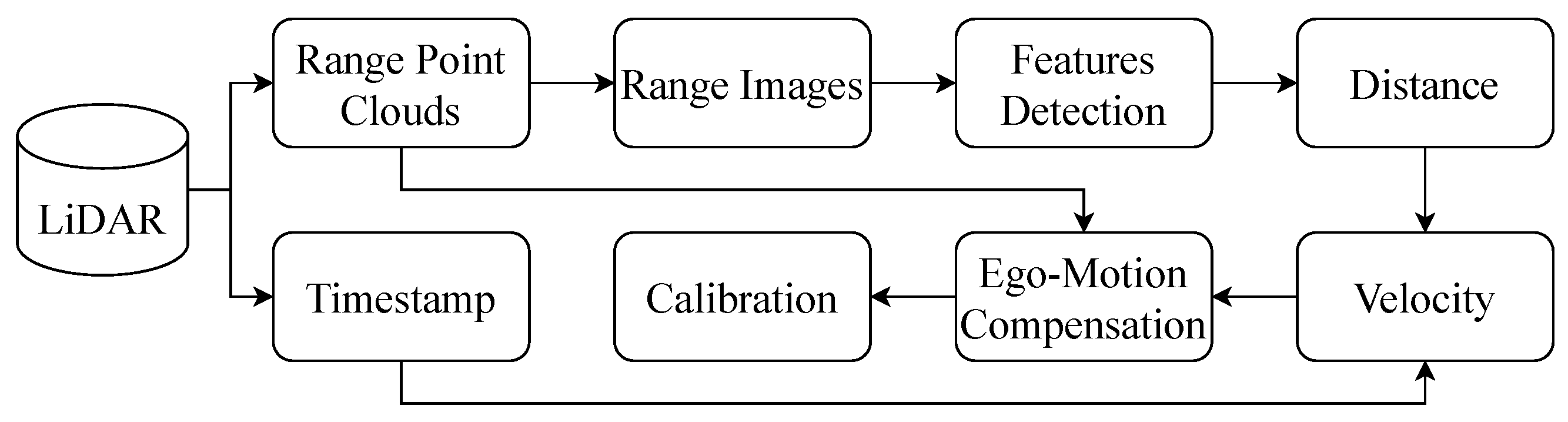
Pipeline of the ego-motion compensation process. First, the point clouds are converted into two-dimensional images using Spherical Projection. Key features are then identified within these range images, and corresponding point pairs are matched. By matching key feature pairs, the distance between frames can be determined, allowing for velocity estimation. Finally, velocity and timestamp will be used to resolve ego-motion compensation and point cloud accumulation.
Figure 14.
Pipeline of the ego-motion compensation process. First, the point clouds are converted into two-dimensional images using Spherical Projection. Key features are then identified within these range images, and corresponding point pairs are matched. By matching key feature pairs, the distance between frames can be determined, allowing for velocity estimation. Finally, velocity and timestamp will be used to resolve ego-motion compensation and point cloud accumulation.
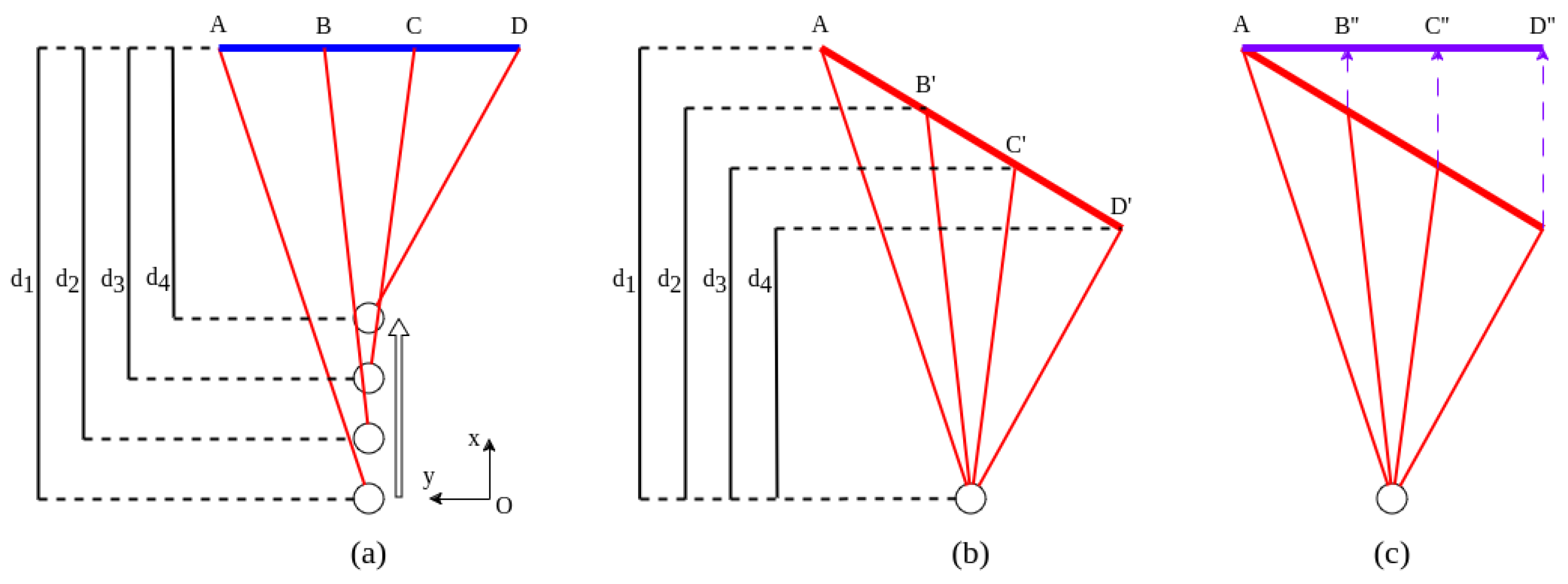
Visualization of distortion correction. The motion of the vehicle is presented by the circles, and the LiDAR is also sotating while the vehicle is in motion. (a) shows the actual shape of the obstacle. (b) depicts the shape of the obstacle scanned by LiDAR. (c) illustrates the shape of the obstacle after distortion correction.
Figure 15.
Visualization of distortion correction. The motion of the vehicle is presented by the circles, and the LiDAR is also sotating while the vehicle is in motion. (a) shows the actual shape of the obstacle. (b) depicts the shape of the obstacle scanned by LiDAR. (c) illustrates the shape of the obstacle after distortion correction.
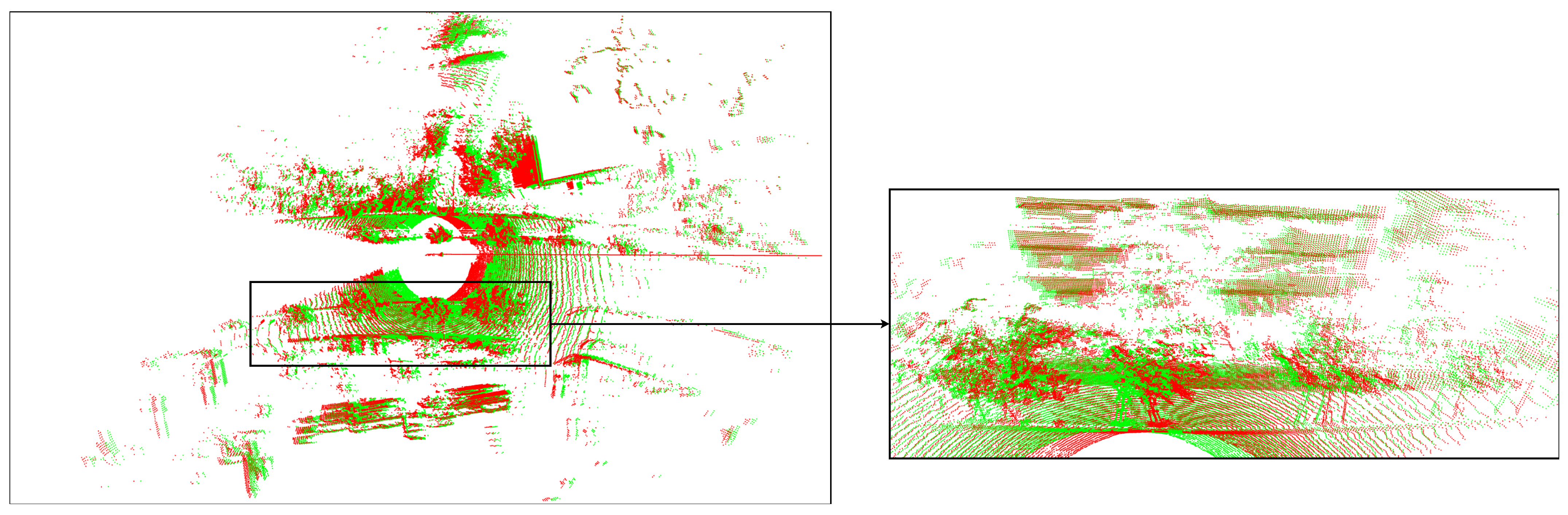
Visualization of the differences in distortion correction on 3D point clouds within a frame with a speed of 54 km/h and a frequency of 10 Hz. The red part shows the original points of the point clouds, while the green part shows the corrected points. The left image shows points on the -plane. The right image shows points on the -plane.
Figure 16.
Visualization of the differences in distortion correction on 3D point clouds within a frame with a speed of 54 km/h and a frequency of 10 Hz. The red part shows the original points of the point clouds, while the green part shows the corrected points. The left image shows points on the -plane. The right image shows points on the -plane.
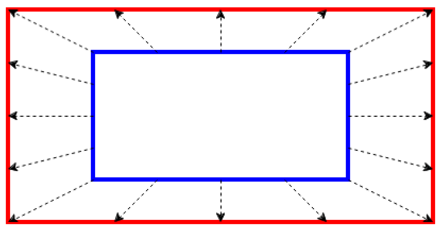
Visualization of distortion correction of cameras. The blue rectangle is the actual shape, and the red rectangle is the shape distorted by ego-motion.
Figure 17.
Visualization of distortion correction of cameras. The blue rectangle is the actual shape, and the red rectangle is the shape distorted by ego-motion.
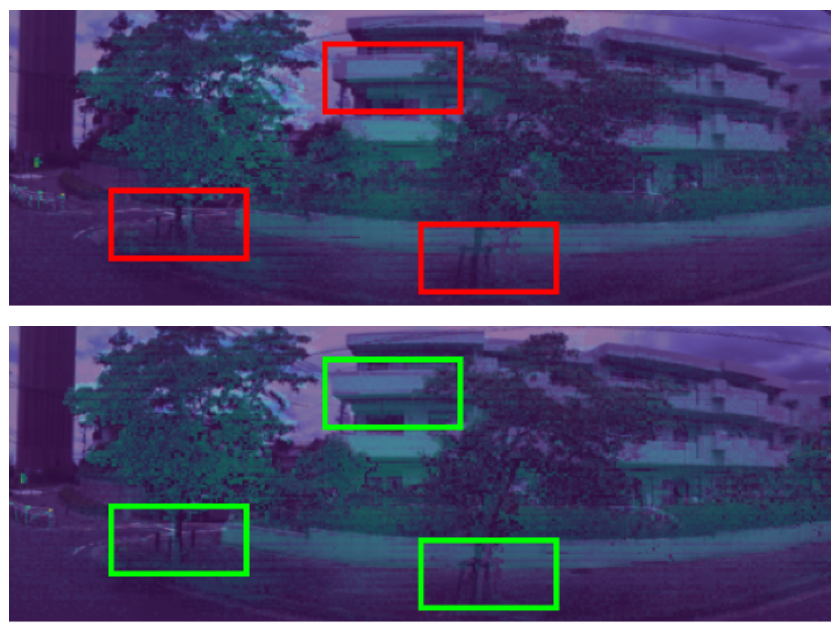
Visualization of 360 RGB–LiDAR images calibration. The (above image) including the red rectangles indicate the calibration results before applying correction. The (below image) including the green rectangles indicates the calibration results after applying correction.
Figure 18.
Visualization of 360 RGB–LiDAR images calibration. The (above image) including the red rectangles indicate the calibration results before applying correction. The (below image) including the green rectangles indicates the calibration results after applying correction.
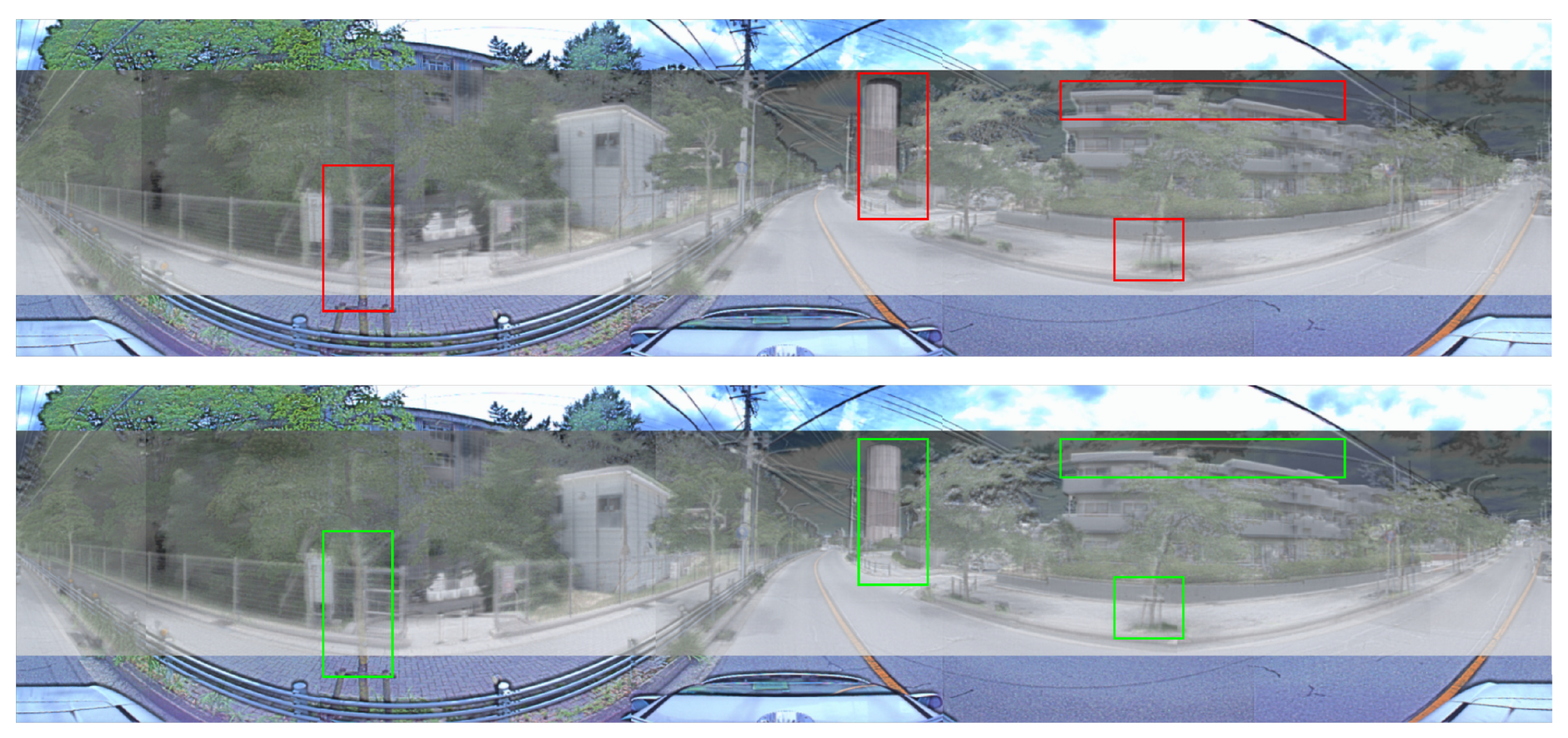
Visualization of 360 RGB–thermal images calibration. The (above image) includes red rectangles that indicate the calibration results before applying correction. The (below image) includes green rectangles that indicate the calibration results after applying correction.
Figure 19.
Visualization of 360 RGB–thermal images calibration. The (above image) includes red rectangles that indicate the calibration results before applying correction. The (below image) includes green rectangles that indicate the calibration results after applying correction.
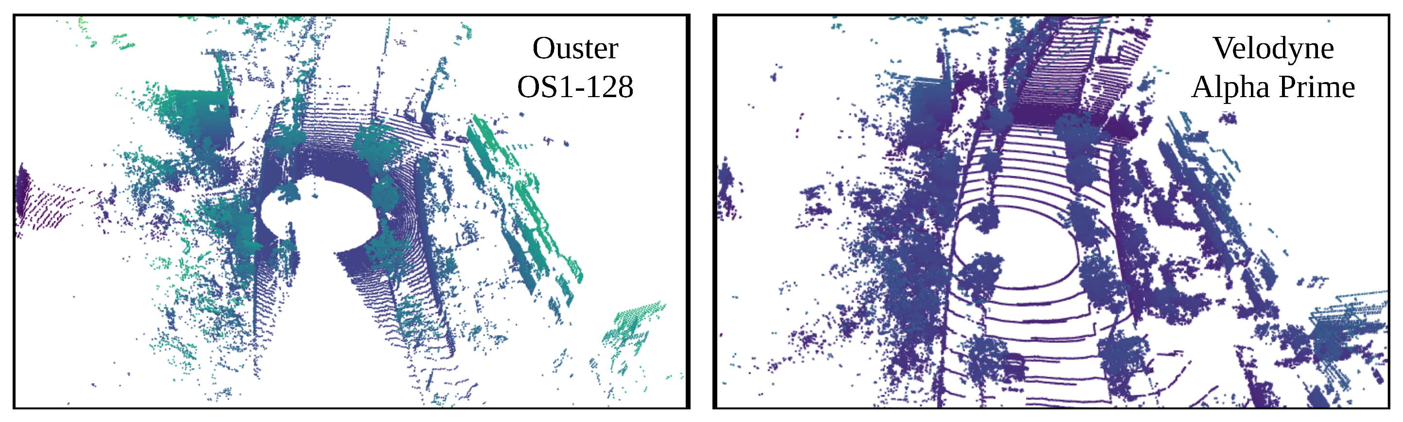
Visualization of point clouds extracted from Ouster OS1-128 and Velodyne Alpha prime.
Figure 20.
Visualization of point clouds extracted from Ouster OS1-128 and Velodyne Alpha prime.
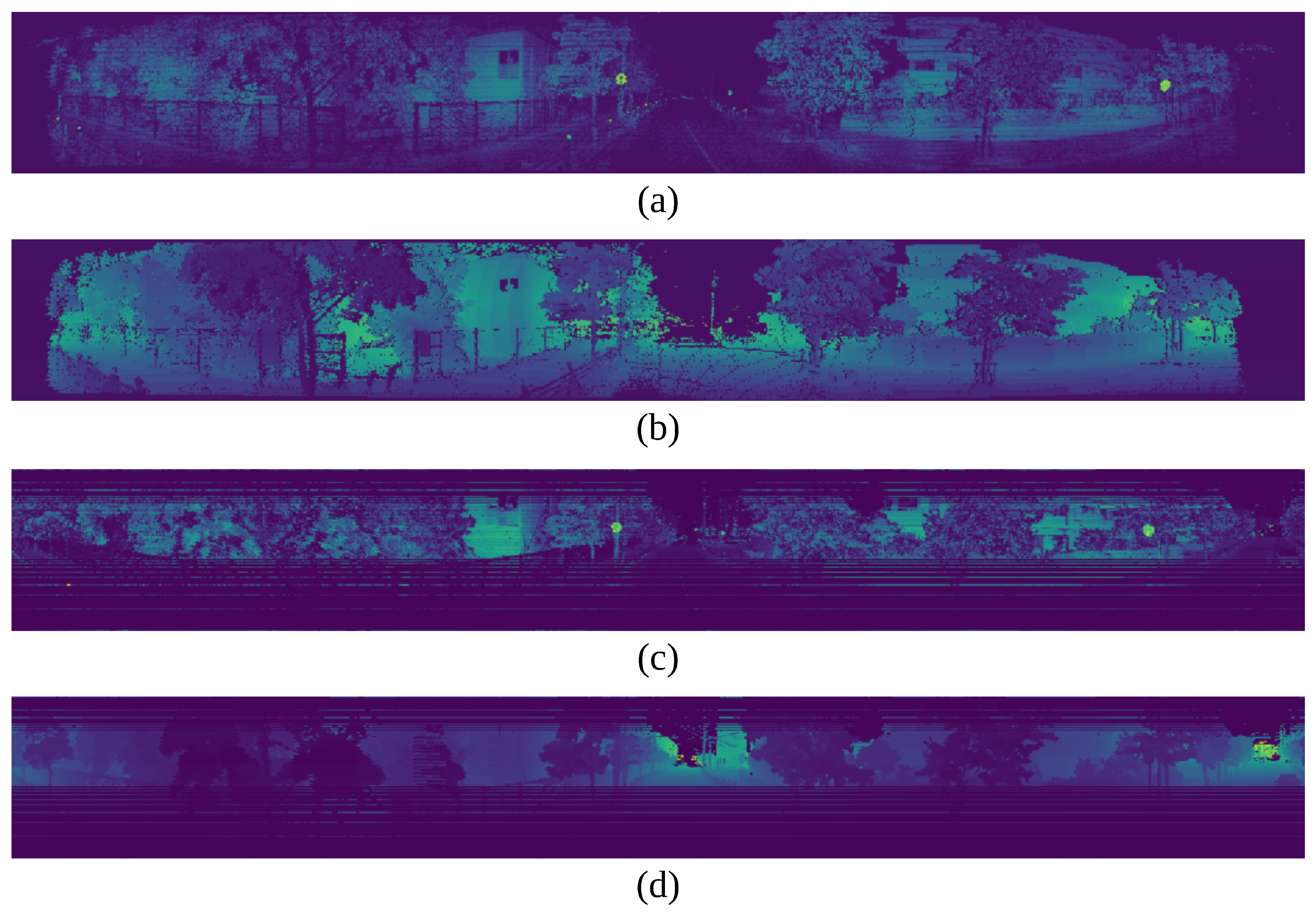
Visualization of image projection. (a) presents the 2D image data with the intensity channel from Ouster OS1-128. (b) presents the 2D image data with the range channel from Ouster OS1-128. (c) presents the 2D image data with the intensity channel from Velodyne Alpha prime. (d) presents the 2D image data with the range channel from Velodyne Alpha prime.
Figure 21.
Visualization of image projection. (a) presents the 2D image data with the intensity channel from Ouster OS1-128. (b) presents the 2D image data with the range channel from Ouster OS1-128. (c) presents the 2D image data with the intensity channel from Velodyne Alpha prime. (d) presents the 2D image data with the range channel from Velodyne Alpha prime.
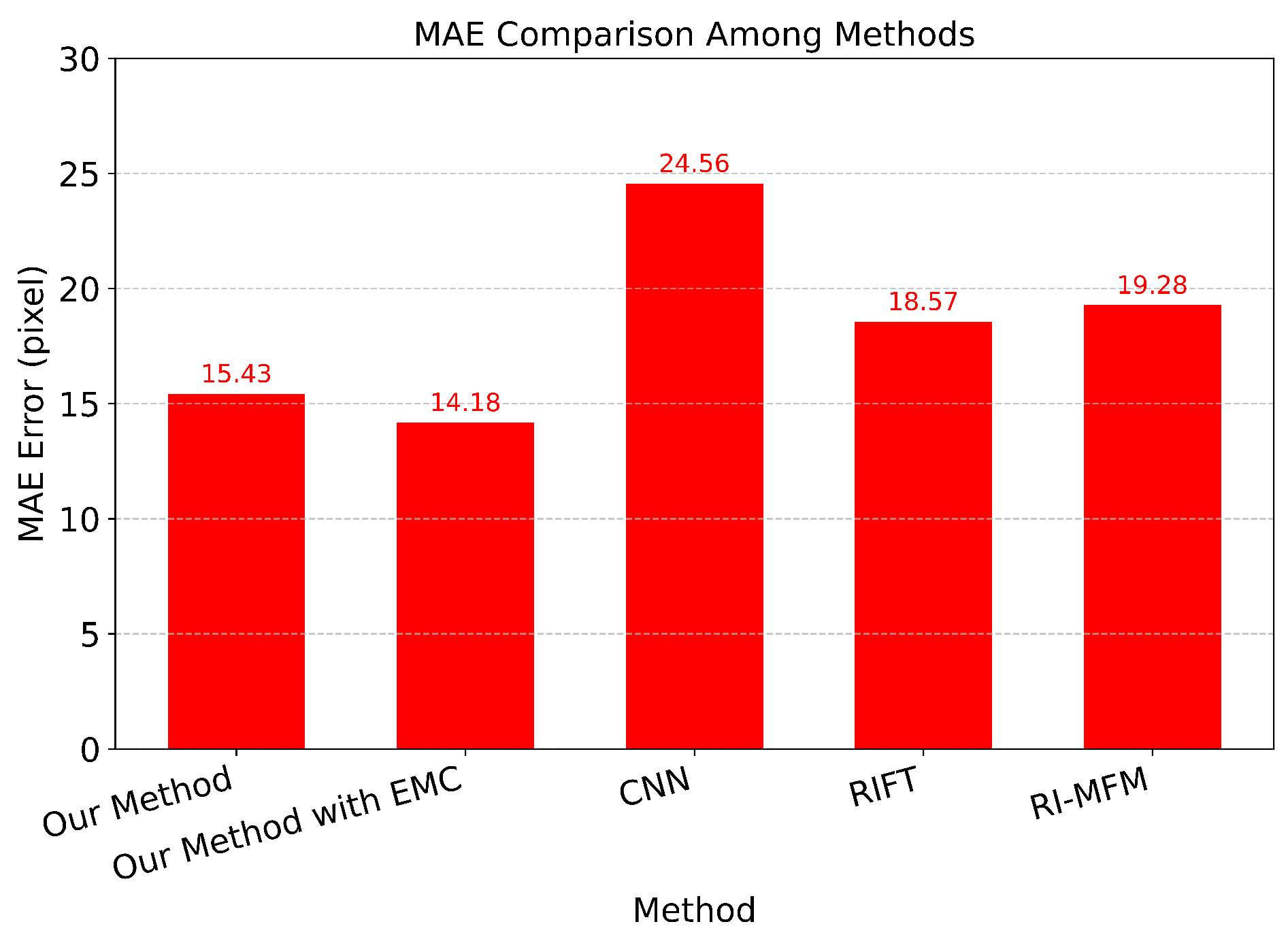
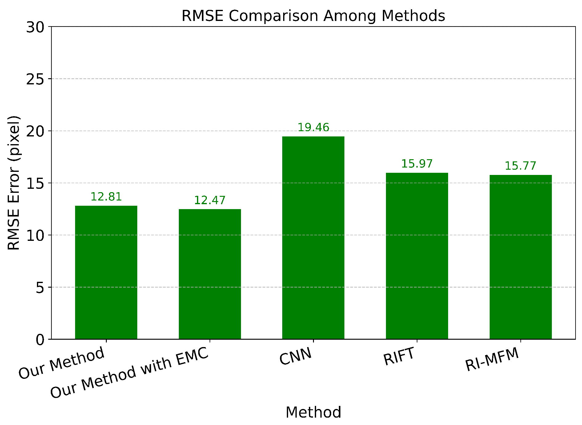
Comparison with CNN, RIFT, RI-MFM by MAE.
Figure 23.
Comparison with CNN, RIFT, RI-MFM by MAE.
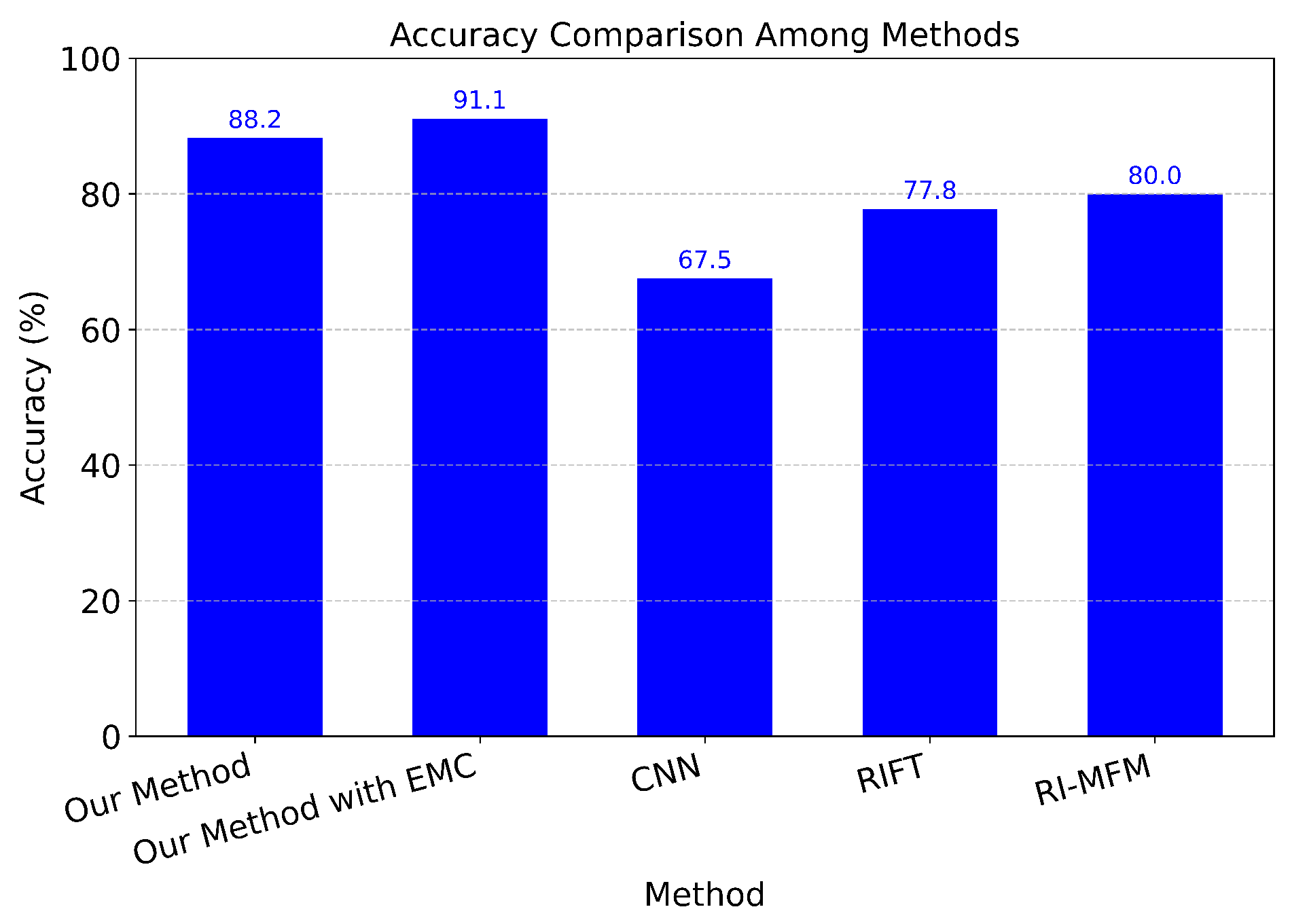
Comparison with CNN, RIFT, RI-MFM by Accuracy.
Figure 24.
Comparison with CNN, RIFT, RI-MFM by Accuracy.
Comparison with CNN, RIFT, RI-MFM by RMSE.
Figure 25.
Comparison with CNN, RIFT, RI-MFM by RMSE.
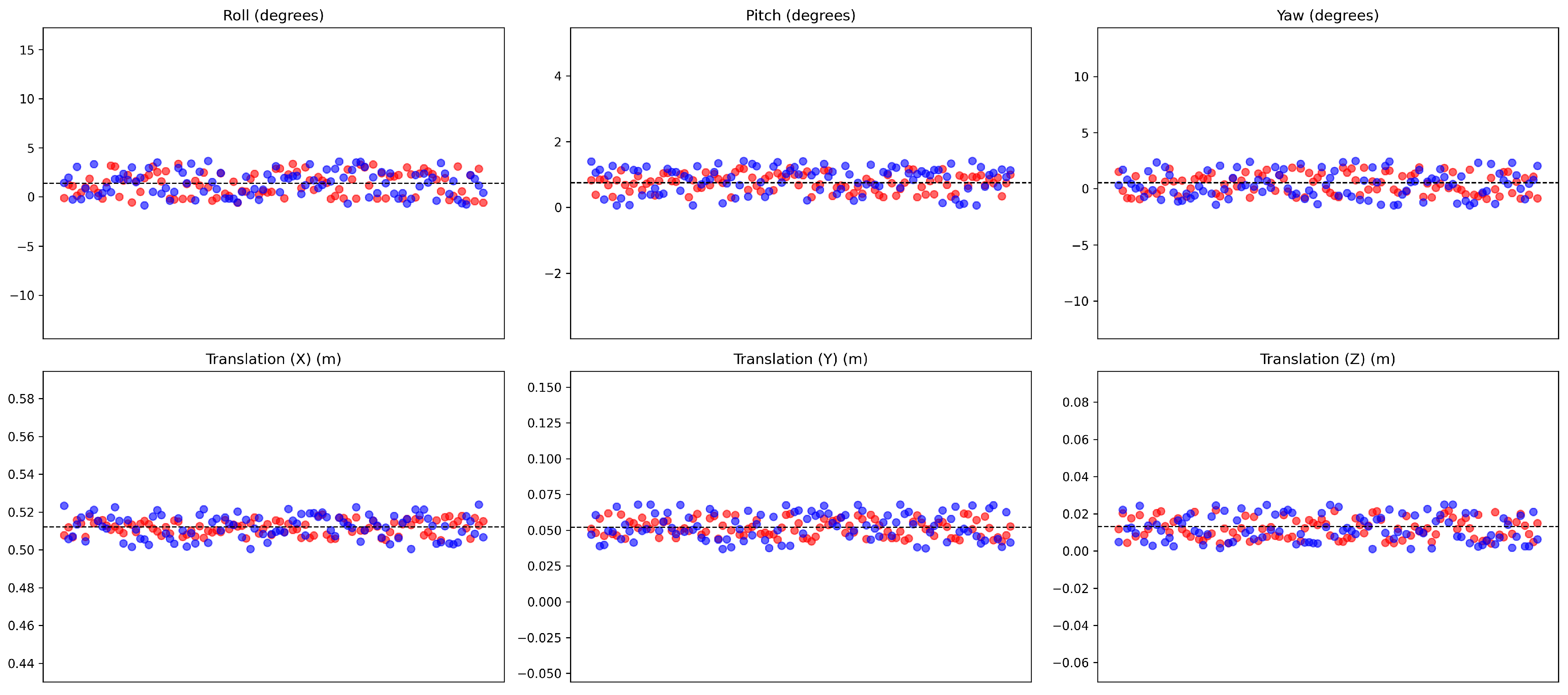
Red points represent the results of calibration without distortion correction, while blue points represent the results with distortion correction in static situations. The dashed line is the results from the target based method.
Figure 26.
Red points represent the results of calibration without distortion correction, while blue points represent the results with distortion correction in static situations. The dashed line is the results from the target based method.
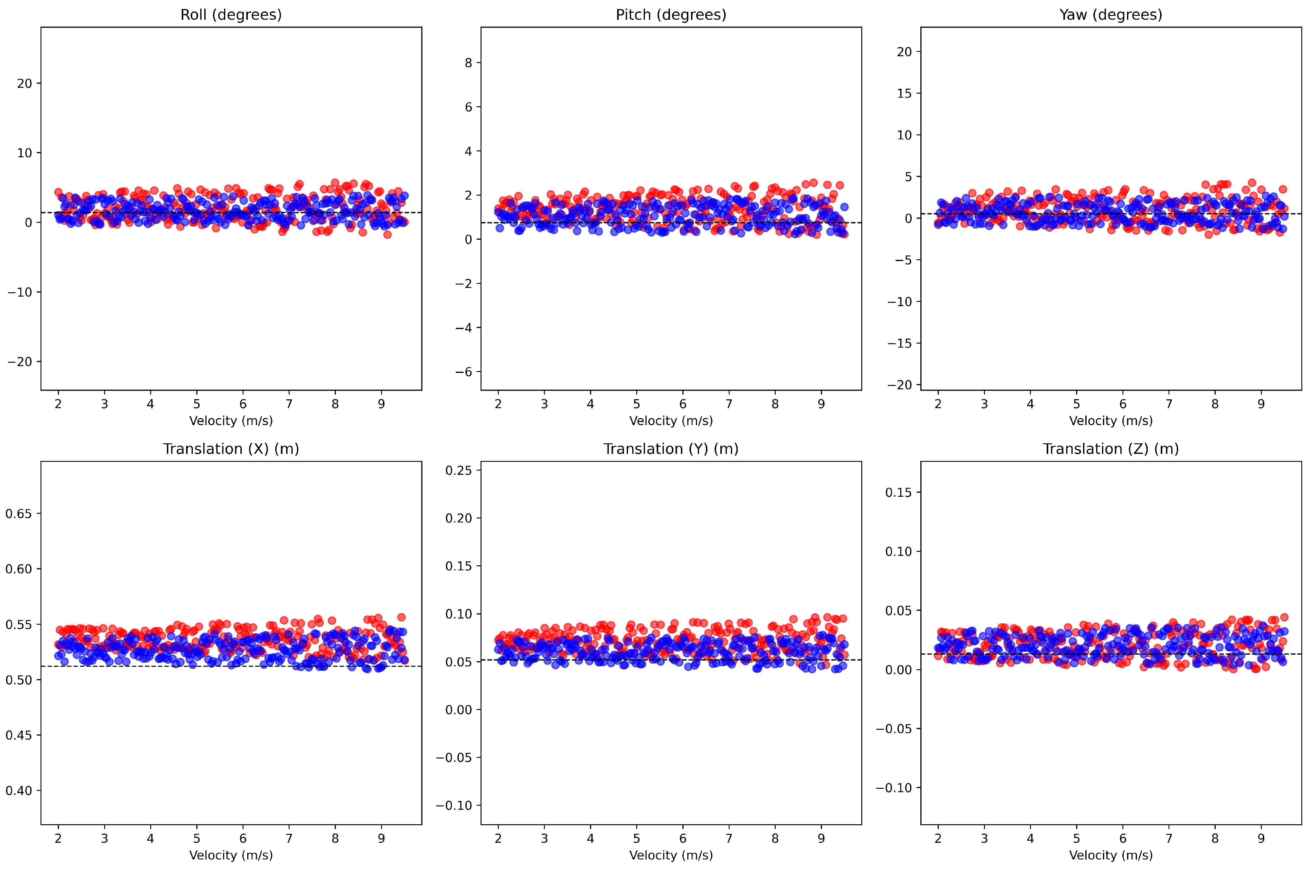
Red points and blue points represent the results of calibration without and with distortion correction in dynamic situations. The dashed lines present the results using the actual data.
Figure 27.
Red points and blue points represent the results of calibration without and with distortion correction in dynamic situations. The dashed lines present the results using the actual data.
Comparison of error in rotation and translation of three methods.
Figure 28.
Comparison of error in rotation and translation of three methods.
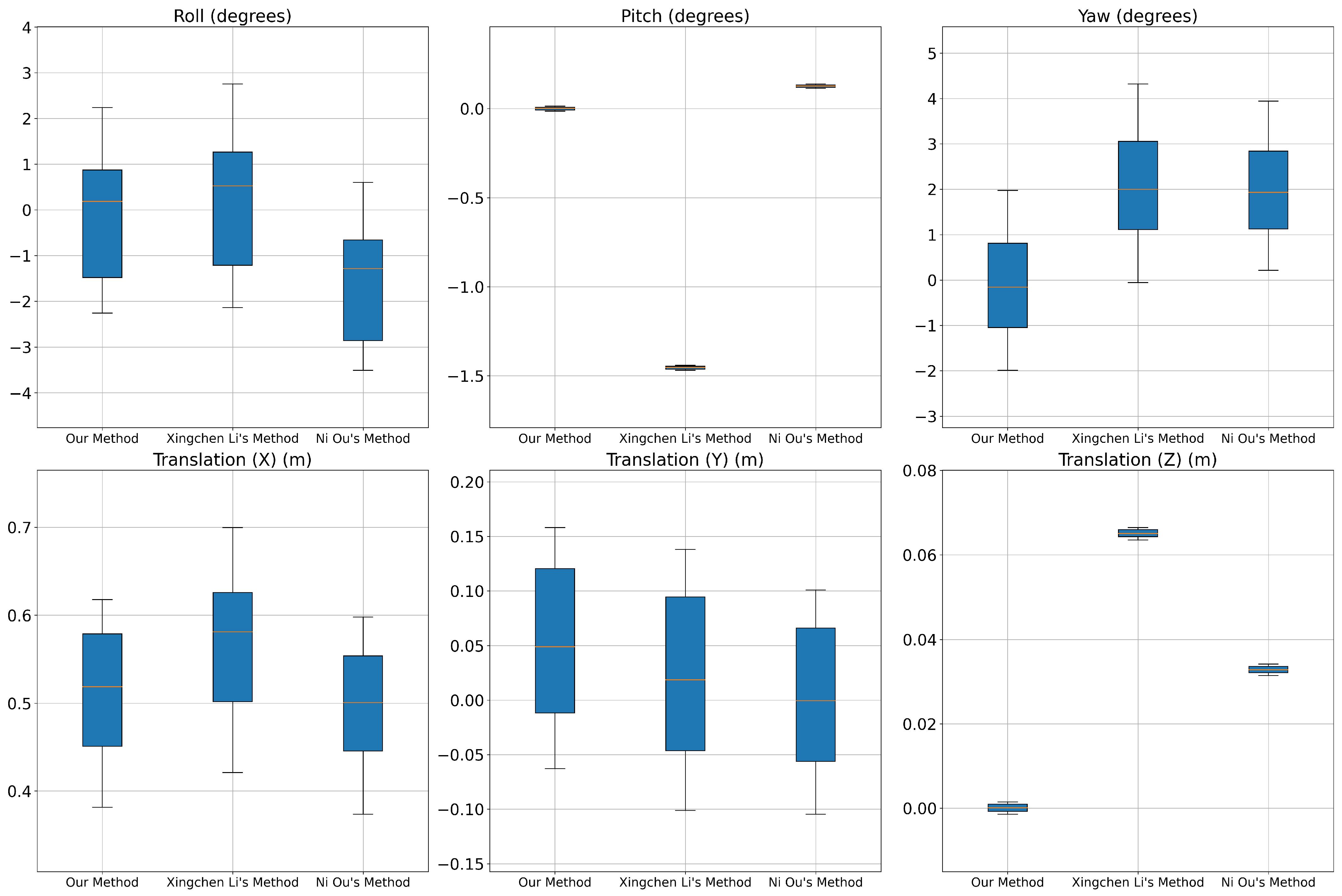
Table 1.
Maximum and average velocity measurements.
Table 1.
Maximum and average velocity measurements.
| Name | Max Velocity | Mean Velocity |
|---|---|---|
| Ouster | 9.51 m/s | 5.56 m/s |
| Velodyne | 9.74 m/s | 5.59 m/s |
| Ground Truth | 9.47 m/s | 5.59 m/s |
Table 2.
Mean errors of targetless calibration in static situations.
Table 2.
Mean errors of targetless calibration in static situations.
| Mean Errors | Without Ego-Motion Compensation | With Ego-Motion Compensation |
|---|---|---|
| Roll Error (degrees) (°) | 1.0714 | 1.0886 |
| Pitch Error (degrees) (°) | 0.2162 | 0.3624 |
| Yaw Error (degrees) (°) | 0.7999 | 1.0015 |
| Translation (X) Error (m) | 0.0032 | 0.0054 |
| Translation (Y) Error (m) | 0.0051 | 0.0081 |
| Translation (Z) Error (m) | 0.0048 | 0.0064 |
Table 3.
Mean errors of targetless calibration in dynamic situations.
Table 3.
Mean errors of targetless calibration in dynamic situations.
| Velocity | Mean Errors | Without Ego-Motion Compensation | With Ego-Motion Compensation |
|---|---|---|---|
| 2 m/s–3 m/s | Roll Error (degrees) (°) | 1.2446 | 1.1996 |
| Pitch Error (degrees) (°) | 0.4448 | 0.3734 | |
| Yaw Error (degrees) (°) | 1.1874 | 1.1131 | |
| Translation (X) Error (m) | 0.0184 | 0.0121 | |
| Translation (Y) Error (m) | 0.0136 | 0.0086 | |
| Translation (Z) Error (m) | 0.0087 | 0.0080 | |
| 3 m/s–4 m/s | Roll Error (degrees) (°) | 1.3190 | 1.2146 |
| Pitch Error (degrees) (°) | 0.5779 | 0.3440 | |
| Yaw Error (degrees) (°) | 1.2619 | 1.1733 | |
| Translation (X) Error (m) | 0.0268 | 0.0152 | |
| Translation (Y) Error (m) | 0.0185 | 0.0093 | |
| Translation (Z) Error (m) | 0.0099 | 0.0082 | |
| 4 m/s–5 m/s | Roll Error (degrees) (°) | 1.3797 | 1.2636 |
| Pitch Error (degrees) (°) | 0.6200 | 0.3866 | |
| Yaw Error (degrees) (°) | 1.3021 | 1.1652 | |
| Translation (X) Error (m) | 0.0239 | 0.0137 | |
| Translation (Y) Error (m) | 0.0210 | 0.0102 | |
| Translation (Z) Error (m) | 0.0101 | 0.0088 | |
| 5 m/s–6 m/s | Roll Error (degrees) (°) | 1.4497 | 1.3053 |
| Pitch Error (degrees) (°) | 0.7387 | 0.4228 | |
| Yaw Error (degrees) (°) | 1.3870 | 1.2093 | |
| Translation (X) Error (m) | 0.0213 | 0.0148 | |
| Translation (Y) Error (m) | 0.0206 | 0.0105 | |
| Translation (Z) Error (m) | 0.0110 | 0.0087 | |
| 6 m/s–7 m/s | Roll Error (degrees) (°) | 1.5521 | 1.2817 |
| Pitch Error (degrees) (°) | 0.6482 | 0.4519 | |
| Yaw Error (degrees) (°) | 1.4743 | 1.2412 | |
| Translation (X) Error (m) | 0.0242 | 0.0157 | |
| Translation (Y) Error (m) | 0.0199 | 0.0108 | |
| Translation (Z) Error (m) | 0.0116 | 0.0094 | |
| 7 m/s–8 m/s | Roll Error (degrees) (°) | 1.6495 | 1.3175 |
| Pitch Error (degrees) (°) | 0.7719 | 0.4841 | |
| Yaw Error (degrees) (°) | 1.6465 | 1.2775 | |
| Translation (X) Error (m) | 0.0236 | 0.0162 | |
| Translation (Y) Error (m) | 0.0189 | 0.0106 | |
| Translation (Z) Error (m) | 0.0132 | 0.0091 | |
| 8 m/s–9 m/s | Roll Error (degrees) (°) | 1.7663 | 1.3422 |
| Pitch Error (degrees) (°) | 0.8377 | 0.5072 | |
| Yaw Error (degrees) (°) | 1.7007 | 1.2710 | |
| Translation (X) Error (m) | 0.0249 | 0.0154 | |
| Translation (Y) Error (m) | 0.0226 | 0.0114 | |
| Translation (Z) Error (m) | 0.0147 | 0.0110 | |
| 9 m/s–9.5 m/s | Roll Error (degrees) (°) | 1.9336 | 1.3637 |
| Pitch Error (degrees) (°) | 0.9996 | 0.5446 | |
| Yaw Error (degrees) (°) | 1.8124 | 1.3053 | |
| Translation (X) Error (m) | 0.0256 | 0.0184 | |
| Translation (Y) Error (m) | 0.0241 | 0.0138 | |
| Translation (Z) Error (m) | 0.0153 | 0.0113 |
Source link
Khanh Bao Tran www.mdpi.com