2.1. Study Area and Sampling
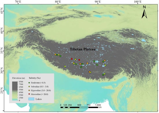
We investigated 25 lakes distributed across an altitude range of 4031~5008 m in July~September 2020 (
Figure 1). These lakes are mostly above the treeline (the average altitude of the alpine treeline in the Himalayas, located on the southern edge of the Tibetan Plateau, is 3633 m [
37]), and lake depths range between 3.8 and 55.7 m, with an average of 21.4 m. The vegetation in most areas consists mainly of alpine meadows or shrubs, with little to no trees around the lakes, or only sparse small plants. The sampled lakes included 9 freshwater lakes (salinity < 0.5‰) and 16 saline lakes. The saline lakes can be further categorized into 8 subsaline lakes (salinity = 0.5‰~3‰), 6 hyposaline lakes (salinity = 3‰~20‰), and 2 mesosaline lakes (salinity > 20‰) (
Figure 1). For each lake, we selected 1~4 sampling sites (more sites in lakes with larger area) located towards the center of the lake, resulting in a total of 44 sediment samples. We avoided sites near the shore to avoid wave disturbance on the sediments. We arrived at the sampling sites by motorboat and used a global positioning system to record longitude, latitude, and altitude. At each sampling site, we collected 2 L of water from the upper 50 cm surface layer by a 5 L Schindler sampler and retrieved the surface sediment at the same location with a 6 cm diameter gravity core. We filtered 1 L of water through glass fiber filter membrane with a pore size of 0.7 µm (GF/F, Whatman) and stored the membranes in the dark at −20 °C until chlorophyll-
a (Chl-
a) analysis. We stored the remaining 1 L water samples at 4 °C until C, N, and P analyses. We carefully collected only the first centimeter of sediments from the sediment cores because the top surficial layer of sediments typically possesses higher microbial cell density, extracellular enzymatic activities (EEAs), and microbial activities [
38,
39,
40]. We well homogenized each sediment sample and separated it into two subsamples. We then stored the two subsamples at −20 °C until analysis. One was used to analyze the composition and diversity of microbial community and to quantify the EEAs, while the other was used to determine the C, N, and P contents. Freezing is a recommended procedure for sediment preservation when the EEAs cannot be determined immediately [
41]. All equipment, tools, and containers used during sediment sampling were sterilized in advance to avoid contamination. Moreover, we used disposable gloves, spoons, and blades for mixing and collecting samples, ensuring that all equipment and tools were carefully cleaned between sample collections. All sampling containers were pre-washed with distilled water and autoclaved before use. In addition, we monitored in situ environmental parameters at each sampling site. Specifically, water depth was obtained by a bathymeter; temperature and salinity in the water column were measured using a multiparameter water quality probe (YSI Incorporated, Yellow Springs, OH, USA).
2.2. C, N, and P Content Determinations
We freeze-dried the surface sediments before chemical and biological analyses. For sediment total nitrogen (TN) and total phosphorus (TP) measurements, we passed the freeze-dried subsamples through a 100-mesh sieve after grinding. We determined the sediment TN using the combustion method by an elemental analyzer (EA 3000, Euro Vector, Pavia, Italy). We analyzed the sediment TP following molybdenum, antimony, and scandium colorimetry [
42]. For TN and TP in water samples, we used persulfate digestion to convert all nitrogen forms and organic phosphorus into nitrate and phosphate, respectively. Subsequently, we quantified the concentrations of nitrate and phosphate using colorimetric methods [
42]. We passed the freeze-dried subsamples through a 10-mesh sieve and mixed them with carbon dioxide-free water at sediment-to-water ratios of 1:5 and 1:2.5 (g/mL). For the first ratio, the mixture was oscillated for 30 min, left for 30 min, filtered to obtain the supernatant, and then measured for conductivity using a conductivity electrode; for the second ratio, the mixture was oscillated for 2 min, left for 30 min, and measured for pH using a pH electrode [
43]. Measuring the pH and conductivity using freeze-dried sediment samples ensured uniformity and comparability across all samples and avoided issues caused by variations in the timing of sample collection. The water salinity, sediment pH, and conductivity probes were calibrated with standard solutions to ensure accuracy and consistency among all samples.
We mixed the freeze-dried sediments with water (1:20 sediment/water ratio, g/mL) and filtered them through a 0.45 µm glass fiber membrane to extract the dissolved inorganic nitrogen (DIN, i.e., NH
4+, NO
3−, and NO
2−), dissolved inorganic phosphorus (DIP, i.e., PO
43−) and DOC in surface sediments. We diluted the solution with ammonia-free water at a ratio of 1:10 and subsequently analyzed sediment DIN and DIP using colorimetric methods. NH
4+ and PO
43− were quantified following the Nessler’s reagent and molybdenum blue spectrophotometric method, respectively. NO
3− was determined directly at 275 and 220 nm light wavelengths, while NO
2− was determined by reacting the sample with Griess reagent to form a colored compound [
42]. We used a TOC analyzer (ET1020A, O.I. Analytical, College Station, Texas, USA) to determine SOC and DOC.
Additionally, we also measured water Chl-
a, which could be used to indicate nutrients and organic matter from algal biomass since algal biomass can support the C acquisition and growth of the microbial community [
44]. Water Chl-
a was measured spectrophotometrically after extraction in 90% acetone following standard method [
45].
2.3. Bacterial and Fungal Community Analyses
We extracted the sediment genomic DNA using the DNeasy PowerSoil Kit (QIAGEN, Hilden, Germany) according to the manufacturer’s protocols. Meanwhile, three blank controls were performed following the same procedures as the sample treatments to control for potential laboratory contamination. For bacteria, we amplified the V4 region of the 16S ribosomal RNA gene using the universal primers [515F, 5′-GTGYCAGCMGCCGCGGTAA-3′ and 806R, and 5′-GGACTACNVGGGTWTCTAAT-3′] via the polymerase chain reaction. For fungi, we amplified the internal transcribed spacer 2 (ITS2) region of the nuclear ribosome using the universal primers [gITS7F, 5′-GTGARTCATCGARTCTTTG-3′ and ITS4R, and 5′-TCCTCCGCTTATTGATATGC-3′]. The PCR amplifications were carried out with the following steps: an initial denaturation at 94 °C for 5 min, followed by 24 cycles consisting of 30 s of denaturation at 94 °C, 30 s of annealing at 56 °C, and 20 s of extension at 72 °C, with a final extension at 72 °C for 5 min. To assess the presence of contamination and validate the amplification process, negative controls (no-template controls, NTCs) were included in each PCR set. The PCR products were then analyzed using 1.5% agarose gel electrophoresis, purified using AMPure XP beads (Beckman, Brea, CA, USA), and quantified with the Qubit dsDNA assay kit using a Qubit 2.0 Fluorometer (Thermo Fisher Scientific, Waltham, MA, USA). The negative controls (extraction blanks and NTCs) were analyzed to detect any potential contamination across the workflow, and no amplification or DNA was detected in these samples. We then normalized the barcoded PCR products of bacterial or fungal samples at equal molar concentration and sequenced them with 2 × 250 bp paired-end on the Illumina HiSeq sequencing platform (Illumina Inc., San Diego, CA, USA).
Finally, we processed the bacterial and fungal sequences on the Quantitative Insights into Microbial Ecology (QIIME, v2.0) pipeline [
46]. Briefly, for bacteria, sequences were denoised to obtain amplicon sequence variants (ASVs) following the processes of removing low-quality and redundant sequences and splicing sequences and removing chimeras with the “DADA2” package [
47]. The specific taxonomic classifier was trained and generated based on the primers used for amplification, the length of our sequence reads, and the preformatted reference sequence and taxonomy for the SILVA ribosomal RNA database using the “q2-feature-classifier” algorithm [
48]. Then, the taxonomy assignment of ASVs was performed based on the specific taxonomic classifier using the “classify-sklearn” algorithm [
49]. For fungi, the sequence processing was the same as for bacteria except that the taxonomy annotation was performed based on the UNITE database [
50]. Finally, both the bacterial and fungal ASVs were rarefied to the minimum sequence number to prevent variations in abundance or sampling intensity from interfering with the biodiversity calculations.
2.4. EEAs Assays
The enzymes we studied were β-1,4-Glucosidase (BG), cellobiohydrolase (CBH), β-1,4-N-acetylglucosaminidase (NAG), leucine aminopeptidase (LAP), and alkaline phosphatase (AP). These extracellular enzymes catalyze the terminal reactions in substrate hydrolysis to acquire C, N, and P. Specifically, BG and CBH catalyze cellulose degradation, NAG and LAP catalyze chitin and polypeptide degradation, AP catalyzes phospholipid and phosphosaccharide degradations. We measured the EEAs of these five enzymes using a fluorimetric microplate enzyme assay [
51]. This method directly measures the fluorescence intensity of products released from the fluorimetrically labelled substrates added to sediment suspensions, eliminating the need for prior extraction and purification of enzymes. This approach allows for the rapid analysis of a large number of sediment samples and enzymes. We used substrates conjugated with highly fluorescent compounds, 7-amino-4-methyl coumarin (7-AMC) and 4-methylumbelliferone (4-MUB), to measure the activities of LAP and four other enzymes, respectively. The water used for incubation was collected in situ for each sample, filtered through 0.2-µm nylon filters to eliminate bacteria and particles, autoclaved to eliminate enzymatic activity, and then kept frozen until it acclimated to the incubation temperature for EEAs measurements. Additionally, sediment turbidity and phenolics affect the fluorescence intensity of 4-MUB and 7-AMC by causing quenching [
52]. The extent of quenching differs across various sediment suspensions, making it necessary to apply a correction procedure for each sediment analyzed. This procedure involves using a specific standard in the same sediment matrix. Consequently, each plate included at least three replicates for each substrate (sample + buffer + substrate), a quenched standard (sample + buffer + 4-MUB/7-AMC), a substrate control (water + buffer + substrate), and an optional abiotic control (autoclaved sediment + buffer + substrate). Incubation was performed using 1 g of sediment samples, 10 mL of previously autoclaved water, and the corresponding substrate for each EEA with a final concentration standardized of 0.2 mM. This concentration was determined based on preliminary experiments, in which different gradient concentrations of the substrate were tested on the same sample to optimize the enzyme reaction. The buffer selection was based on the specific enzyme being tested. BG, CBH, and NAG were measured using 0.1 M MES buffer (2-[N-Morpholino]ethanesulfonic acid, pH 6.1), AP was assayed in 0.1 M MES buffer at pH 10, and LAP was tested in 0.05 M Trizma buffer at pH 7.8. After a 30 min incubation in the dark on a shaking table at an average ambient temperature of 15 °C (ranging from 12 °C to 19 °C during sampling), the reaction was stopped using sodium hydroxide solution (1 M) before measuring the fluorescence, then the fluorescence emission from the AMC or MUB product was quantified using a computerized microplate fluorimeter (SH1M-SN, Agilent BioTek), with excitation/emission wavelengths set to 364/445 or 365/455. The EEAs were expressed as nanomoles of AMC or MUB released per gram of dry sediment per hour (nmol g sediment
−1 h
−1).
2.6. Statistical Analysis
Our analyses intended to explore (1) the variations in MMLs along lake salinity, and the impacts of nutrients and microbial diversity on these variations, and (2) the correlations between MMLs and SOC. To achieve goal (1), we explored the following three aspects: the variations in MMLs, nutrients and EEAs across lake salinity gradients; potential drivers influencing microbial diversity; and the impacts and respective contributions of salinity, nutrients, and microbial diversity to MMLs.
For the first aspect, we used the linear regression to analyze the relationships of lake salinity with MMLs, sediment nutrients (i.e., SOC, TN, TP, SOC:TN, and SOC:TP), EEAs, and enzymatic stoichiometry (i.e., the C, N, or P acquisition EEAs and their proportions to total EEAs, the stoichiometry ratios between C, N, and P acquisition EEAs). All variables were log-transformed prior to these analyses in order to satisfy the assumptions of linear regression, such as normality and homoscedasticity. We further used analysis of variance (ANOVA) to compare MMLs and other environmental factors between freshwater, subsaline, hyposaline, and mesosaline lakes. Since sediment pH was suggested to be a key driver of MMLs, we also performed linear regression to analyze the relationships of sediment pH with MMLs, sediment nutrients, EEAs, and enzymatic stoichiometry.
For the second aspect, we quantified the relative contributions of environmental factors to microbial species richness using random forest [
53]. We then examined the significance and predictive power of geographic distance and multiple environmental factors in explaining bacterial and fungal community composition differences using multiple regression on dissimilarity matrix (MRM) approach. This approach allowed us to identify linear, nonlinear, or nonparametric relationships between a community dissimilarity matrix and any number of explanatory distance matrices [
54].
For the third aspect, we quantified the relative contributions of each environmental factor and microbial diversity to MMLs using random forest analysis. The microbial diversity included the richness of bacteria and fungi and the community structure of bacteria and fungi represented by the first axis of detrended correspondence analysis of the communities (DCA1). In addition, we partitioned the explanatory variables into the following five main driver categories: climatic factors, geographical features, pH and salinity, nutrients, and microbial diversity. Climate factors included the annual mean temperature (MAT) and annual mean precipitation (MAP), which were downloaded from the CHELSA dataset (Climatologies at high resolution for the Earth’s land surface areas,
https://chelsa-climate.org) [
55,
56]. These data were then extracted based on the longitude and latitude of the sampling sites using the R package “raster V3.6-31”. The geographical feature was the elevation, with the geographic distance calculated from the longitude and latitude as an additional geographical feature input to the MRM analyses of bacterial and fungal community structures. Nutrients included TN, TP, TN:TP ratio, and Chl-
a in water and TN, TP, SOC, NH
4+, NO
3−, NO
2−, DIP, DOC, SOC:TN ratio, SOC:TP ratio, and TN:TP ratio in sediments. Since no significant effects of climatic and geographical factors on microbial C or N/P limitations were found according to the random forest analyses, these two abiotic factors were excluded from the following analyses. For the remaining three driver categories, we further quantified their pure/shared effects and direct/indirect effects on MMLs by performing variance partitioning analysis (VPA) and partial least squares path modeling (PLS-PM), respectively. VPA partitioned the variation in MMLs into components explained by the above three categories and their shared effects [
57]. PLS-PM offered a framework to analyze the interrelationships among a set of variable blocks, including MMLs and the above three categories, taking into account prior knowledge of the phenomenon being studied [
58]. In the PLS-PM, we performed an ANOVA to estimate the significance of the standardized path coefficient (β) and the model. The standardized total effect of each driver category on MMLs was then calculated from β values, encompassing both direct and indirect correlations.
To achieve goal (2), we used the linear regressions to analyze the correlations between MMLs and SOC. We further fitted the partial linear regressions between MMLs and SOC by controlling for water salinity or sediment pH in order to disentangle the potential control of water salinity or sediment pH on the correlations between MMLs and SOC. Before performing the random forest, VPA, and PLS-PM analyses, potential predictors were selected based on the high variance inflation factors (>10) to avoid strong collinearity or multicollinearity, using the R package “usdm V1.1–18” [
59]. The predictors were Z score-transformed to allow comparisons in the MRM and PLS-PM analyses. The OLS regression, random forest, MRM, VPA, and PLS-PM analyses were conducted with R packages “car V3.1” [
60], “randomForestSRC V3.2.2 [
53]”, “ecodist V2.0.9 [
61]”, “vegan V2.6” [
57], and “plspm V0.5.0” [
58], respectively.