1. Introduction
The interaction between waves and vessels such as ships can be complex, resulting in global vessel motions and hull deformations, including vertical bending and often torsion. These actions, which are resisted by the vessel and able to generate global and local stresses (internal actions), are of interest for the design of new vessels and for the condition assessment of older vessels. Ship motions and resulting stresses can be estimated using simplified computational techniques, as typically used for the design of conventional ships with assumed linear response behaviour for low-to-moderate wave heights. Strip theory and panel methods efficiently provide solutions for these load cases [
1,
2,
3,
4]. Another approach is to employ model experiments using a scale version of the vessel of interest subjected to a scaled sea state in a wave towing tank [
5]. Obtaining an estimate of internal actions requires the model to have a degree of flexibility. In model tests, this can be achieved through a model consisting of rigid segments of the hull joined by discrete semi-flexible joints. At these joints, measurements of internal actions can be made [
6,
7,
8,
9]. This approach is used widely for the provision or validation of ship design data, but it is expensive and time-consuming as it may require many physical test runs to obtain information about the effect of different sea states and of different hull options.
Non-linear vessel responses can arise from green water on deck, slamming, bow or stern emergence, and complex or novel hull forms. To accurately predict such non-linear responses requires advanced theoretical models and complex physical models [
10,
11]. For these reasons, increasing attention has been given to numerical modelling. A range of computational fluid mechanics methods and techniques have been developed, with differing degrees of accuracy and areas of application [
1,
2,
12]. One advantage of numerical methods is that, in principle, they should be quicker, cheaper, and have greater repeatability than physical tests.
Within numerical modelling efforts, one approach is that which employs mesh-free particle-based fluid dynamics, typical of a Lagrangian approach [
13]. In this, the fluid domain is represented by a large number of particles. These are taken to have some degree of interaction (see below) so as to accurately represent the fluid motion. One of the more developed mesh-free techniques is that of Smoothed Particle Hydrodynamics (SPH). SPH was initially developed and applied for studies in astrophysics [
14], followed by modifications to account for fluids [
15], and later coupled with solid mechanics components modelled using finite element (FE) solvers, all within a single general purpose software suite [
16,
17]. The coupling of SPH with FE solvers in the single software suite enabled the convenient numerical simulation of many industrial fluid–structure interaction scenarios, including the study of ships at speed in waves [
9,
18,
19,
20,
21,
22]. In the following, this coupled suite is termed SPH-FEA.
The present work is novel in that it uses the said general purpose software suite to generate the waves in SPH and establishes the consequent response of the vessel or ship, using FEA, via the quasi-continuous coupling of the fluid and the vessel. As these are numerical schemes, the coupling is not continuous but occurs at discrete time intervals determined by the timestep of the simulation. In the case presented here, the frequency of coupling was determined by the timestep of the SPH material and was approximately 1000 times a second. The coupling of the fluid and the vessel was enacted by physical forces between the vessel and the fluid at the locations of vessel contact with the discrete SPH particles of the fluid. The response of the vessel is the reaction of the vessel structure to the time-varying distributed forces on the hull from the SPH particles. The current application goes beyond the use of SPH to model ship or other vessel response merely as a rigid body [
22,
23,
24], and instead evaluates the stress within the flexible finite element (FE) structure in relation to the frequency of the coupling [
25,
26].
The SPH-FEA technique has gained increased practical attention in recent years [
18,
19,
20,
21,
22,
23,
24,
25,
26,
27,
28]. One reason for this increased interest is the potential ability of SPH-FEA to represent the complex interaction between waves and structures, particularly when the structure (vessel, ship) is moving and undergoes non-linear deformations under dynamic loading [
24,
28]. Another reason for the recent increased interest is that the high computational requirement of the SPH-FEA technique is becoming more affordable as the cost of computing reduces over time.
The present paper focusses mainly on a comparison of the results achieved by SPH-FEA for a vessel in the form of a naval ship against the results previously reported [
7] for a segmented physical model of that vessel experiencing a head sea wave train incident in a physical wave tank. The details of the physical model and the observed outcomes are available [
7] and were used for selected comparisons in the numerical analyses described herein.
The next section describes the finite element (FE) modelling of the vessel in general terms, followed by an outline of the SPH modelling that was employed. This is followed by a description of the validation of the coupled SPH-FEA approach relative to the results reported for the wave tank experiments. This is completed in three parts. The first part examines the use of the so-called ‘moving floor’ approach to model the generation of water waves as an alternative to the conventional notion of waves generated by a paddle. The second part shows that, even for extreme wave conditions, there are insignificant differences in results between the vessel modelled as a rigid, segmented body mimicking the physical model and as a fully flexible elastic body for the ship and conditions considered here. From this, it is concluded that further comparisons between the physical model results and those from SPH-FEA can be made using the ‘fully flexible’ model for the vessel as it provides a more comprehensive picture of the stress state of the vessel. The ‘fully flexible’ model of the vessel is then used in subsequent comparisons with the results from the physical experiments. These are considered in the sections that follow. Comments are then made about computational effort, future work to improve the results, and the relevance of the present work to fleet asset management. Conclusions close the paper.
2. Numerical Modelling
2.1. Vessel FE Model
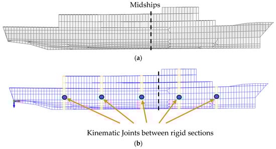
For the present project, the FE model of the vessel considered was made available by the owner. It is elastic and fully flexible. Its veracity was checked against information available for the prototype. This included member steel properties, beam orientations and cross-sections, and plate orientations and thicknesses. Point masses were used to account for machinery, other equipment, fluids in tanks and stores, etc., for a fully laden vessel. In the following, this model is referred to as the ‘fully flexible’ FE model (
Figure 1a).
As noted above, to allow direct comparisons with the results reported for the wave tank experiments, a suitable segmented FE model of the vessel, consistent with the segmented scale wave tank model, was required. This was developed directly from the fully flexible FE model (
Figure 1a) to obtain the segmented FE model (
Figure 1b), as follows.
The fully flexible FE model was modified by dividing it into segments. Each segment was defined as a rigid body, with mass and inertia properties derived from the fully flexible model. Kinematic couplings were used to join the rigid segments to produce a segmented model. The rotational stiffnesses of the kinematic couplings were chosen to ensure that the first vertical bending mode of the segmented model matched that of the fully flexible FE model.
As shown in
Figure 1a,b, the fully flexible and segmented FE models featured identical external shell elements. Unlike the fully flexible FEA model, the segments in the segmented model, being rigid bodies, do not require FEA modelling, and so this represents a small computational saving.
Because the segmented FEA model was required to be merged numerically with the water represented by the SPH modelling, allowance had to be made to prevent water ingress at the couplings. This was undertaken by adding water-impervious flexible shell elements of zero stiffness between the rigid segments (i.e., equivalent to using a flexible membrane between the segments of the physical model).
It should be noted that the precise modelling details of the fully flexible FE model and the segmented FE model are not required for the following analyses since the basic information is the same, apart from the overall modelling of the vessel as fully flexible or segmented. In both cases, the same information was used. As noted, the veracity of the FE model in representing the prototype vessel was checked as part of the present project (and also had been independently confirmed).
2.2. SPH Wave Model
To obtain information about the response of the vessel to wave loading, numerical simulation of the wave loading environment is required. This can be undertaken using SPH, with modelling accomplished using a ‘numerical wave tank’. This is a digital version of the physical wave tank used in the model experiments to obtain the physical response of vessels. Typically, such tanks have a mechanically driven paddle at one end to create circular water motion within the adjacent water column that then propagates to create wave trains with, at the other end of the tank, a beach to dissipate the arriving waves, rather than have them reflect after traversing the length of the tank.
The numerical wave tank dimensions used in the SPH simulation reported herein are listed in
Table 1. For the numerical simulations, the dimensions were verified as providing a sufficient number of wave encounters to establish a steady response, to avoid side wall interference, and to ensure blockage was not significant at the operating conditions of interest [
17]. For convenient correlation to the ship, the tank dimensions were also normalised by the length of the vessel (L).
While the direct simulation of paddle-driven wave tanks is intuitively obvious, it is computationally demanding due to the depth required to ensure deep-water conditions for the wavelengths of interest, and can be challenging over the long lengths required for measuring ship response [
29,
30]. An alternative arrangement for wave generation is the so-called ‘moving floor’ technique [
29].
In the ‘moving floor’ technique, a shallow depth of a deep-water wave is modelled as a sub-domain, as shown in
Figure 2a [
29].
Figure 2b shows a schematic of the sub-domain concept developed for finite elements. It is noted that the sub-domain is extended for many wavelengths and that the lower boundary of the sub-domain is represented by the floor of the tank, and this floor is represented by numerous shell elements per wavelength. Each shell element of the floor in
Figure 2b is prescribed orbits with time in a phased manner relative to an origin, mimicking the orbits inside a deep-ocean wave at that depth. The depth of the moving floor is less than half a wavelength to ensure orbits of effective radius for generating surface waves.
The theory of the moving-floor technique has been developed [
31] based on the concepts presented in
Figure 2a [
29]. The moving-floor theory [
31] explains how a surface wave amplitude can be generated that is much larger than the moving-floor amplitude under specific conditions that coincide with resonance. The precise conditions of resonance are dependent upon the viscosity of the fluid, the wavelength, and the tank depth [
32]. This implies immediately that water orbits at a depth greater than the moving floor need not be simulated, and therefore the method is particularly suitable for the deep-water wave conditions of most practical interest.
Figure 3 shows the surface waves developed in a numerical tank using the moving-floor technique. The waves commence development at the right-hand end of the tank and take a few periods to fully develop as they propagate to the left. Beaches at the up- and down-stream ends of the tank minimise the reflection of the wave.
For the present SPH-based study, the water was modelled using SPH particles of 1.2 m diameter. Although relatively large, this was found by experience to provide acceptable accuracy relative to the computational effort [
26]. The relationship between wave height and floor orbit diameter is largely linear for a given wavelength but is also dependent upon the effective viscosity of the SPH fluid [
31,
32]. The diameter and numerical parameters of SPH can influence the effective viscosity, and so the exact relationship between floor motion and surface is complex. A specific wave height was reliably able to be achieved within a few percent by conducting two or three trials of different floor amplitudes. Vivanco et al. [
31] compared the results of the moving floor to the Airy wave theory [
33] in terms of surface profile and velocity distribution with depth at a wave height of 1.5% of wavelength. They found that the correlation in surface profile was excellent, and that the correlation in velocity profile with depth was excellent for a viscosity comparable to water, but the correlation deviated as the viscosity of the fluid increased to 100 or more times that of water. This is not surprising, as Airy wave theory is an inviscid theory.
A further favourable characteristic of surface waves generated by the moving-floor technique is that the wave front becomes steeper than the back of the wave as wave height increases for a given wavelength. This is shown in
Figure 4 for waves of varying steepness travelling from left to right. This asymmetry of the wave is not described by the Airy wave theory but is a characteristic of actual ocean waves up to the point of breaking. The SPH waves were found to break at a similar wave steepness to ocean waves.
The particle velocities within the SPH wave generated by the moving floor are compared to the Airy wave theory velocities in
Figure 5 and
Figure 6.
Figure 5 shows the normalised horizontal velocities at the crest and trough, and
Figure 6 shows the normalised vertical velocities at the mean water level (or zero-crossing point) either side of the crest. In
Figure 5, at the crest and trough, the SPH surface horizontal velocities show good agreement with the Airy wave theory velocities and show a higher velocity than the theory at about 5% of normalised depth, coming back to good agreement at about 15% normalised depth. In
Figure 6, the vertical velocities at the mean water height on either side of the crest show good agreement at the surface, then tend to drop below the Airy wave theory values below the surface. These velocity deviations from Airy wave theory align with those predicted by the moving-floor theory [
31] and are shown to increase with the viscosity of the fluid, agreeing with the trends of depth shown here of the SPH particle velocities. How these discrepancies might influence the response of a ship on the surface travelling at speed has not been investigated.
2.3. Coupling of SPH and FEA Models
To carry out the simulations noted above involving both SPH and FEA to simulate the response of a vessel to different sea states, a suitable FE solver and also a suitable SPH solver must be available. It is also crucial to have an interface between these two solvers to couple the numerical SPH model of the water and water waves with the numerical model for the FE representation of the vessel. For the present project, all these were available in a software package called Virtual Performance Systems, or VPS (myesi.esi-group.com) [
17]. The solvers within that package are integrated, permitting continuous, and likely efficient, simulation of the desired fluid–structure interaction.
In the VPS package, the interface between the vessel and the water is handled using an industry-standard ‘contact interface algorithm’ [
17]. This algorithm defines the physical interaction of the SPH particles with the wetted (mainly immersed) surfaces of the vessel in terms of friction, pressure, and compressibility. A cross-section of the tank boundaries, fluid (particles), and vessel is shown in
Figure 7 at an instant when the vessel is moving vertically normal to the section. It is noted that the SPH particles are not uniformly spaced. This is because they move as they interact with each other and with the vessel (and vice versa). Importantly, the algorithm for the contact surface interface ensures that the SPH particles cannot penetrate the hull surfaces of the vessel nor the tank boundary surfaces.
Corresponding to the orientation of the vessel in the physical towing tank, for the numerical modelling, the vessel was assumed to be oriented along the centreline of the tank. To simulate the vessel velocity relative to the water, the vessel was assumed to remain stationary along that centreline, with the water and the walls (boundary conditions) of the tank moving at the speed desired for the vessel.
Throughout the simulation, the computer results for the parameters describing ship motion and structural response under the applied wave conditions were saved to an output file for use in subsequent analyses. The simulation outputs also provided the basis for various graphical plots, including ship motion and the generalized forces (bending moments, shears) at the locations of the kinetic couplings between the rigid segments of the model hull.
Elsewhere along the hull, these parameters were obtained by interpolation and extrapolation. From these, interior stresses and strains could be determined at particular locations for direct comparison with these parameters as estimated and reported (Morris et al. 2010 [
7]) for a fully flexible vessel.
2.4. Validation of SPH-FEA Modelling Approach
The approach of integrating SPH with FEA outlined above, together with an interface algorithm as available in industry-standard software [
17], has been shown to provide acceptable results for modelling different scenarios [
16]. This experience was utilised for the present project as providing a degree of in-principle validation. However, for the present project, a systematic validation of the SPH-FEA technique for the interaction of wave loading and vessel responses was considered necessary. It was carried out in three steps, as indicated in
Figure 8.
In this step, the iterative process of achieving the desired wave height was conducted for each wave height and wavelength of interest. That is, the floor orbit radius to achieve a specific surface wave height was determined for each wave height and wavelength of interest. A tolerance of the numerical wave height being within 5% of the desired wave height was considered acceptable. This was considered acceptable to ensure non-linearities would still be evident after the non-dimensionalising of all results.
The wavelength of the surface waves for all conditions was the same as the floor excitation wavelength due to the physics of the resonance condition. Hence, no tuning of the wavelength was required.
This step was aimed at assessing how well the response of the vessel (pitch, heave and bending moments) in the segmented FE model compared with the response of the vessel when modelled as fully flexible for the FE implementation. To test this, it was considered that any discrepancies between the two models would be most apparent at demanding operating conditions. For this purpose, one wave condition was analysed for each case with the parameters of (a) Froude number Fr = 0.38, corresponding to 24 knots for the actual vessel, (b) wavelength λ/L = 1, and (c) a wave height of 4.1% L. The nominated wave height is large compared to the length of the vessel and was constrained by the observation [
7] that for the nominated vessel speed of 24 knots, a larger wave height would result in excessive water on deck at model scale. Such a scenario is outside the domain of the simulations considered herein.
It might be noted here that in naval architecture terminology, the Froude number Fr (as used here) indicates the rate of wave propagation (velocity) of an object moving though water [
34] and is defined below.
| Froude Number | | Fr = Froude number (velocity) |
| = flow speed January |
| g = acceleration due to gravity January |
| L = length of the ship January |
After demonstrating (again) the veracity of the moving-floor technique and demonstrating the close equivalence of simulation responses produced by the segmented FE model and the fully flexible FE model for the ship, Step (3) compares various aspects of the response of the vessel as simulated by SPH-FEA against those measured in the segmented physical model [
7]. For this purpose, several different operational scenarios were examined, corresponding to what was reported for the physical model. In all cases, the Froude number was Fr = 0.28, corresponding to 18 knots. The effects of wave height and wavelength were examined, as reported further below.
4. Discussion
In general, the numerical results obtained using the fully flexible FE model for the vessel have similar trends and magnitudes to the results reported and interpreted for the physical segmented scale model vessel in the physical wave tank [
7].
However, the simulated response predictions for heave and pitch, while showing the expected functional relationship with wavelength, showed lower values than those obtained from the physical wave tank experimental results. It is noted that a generally similar disparity was observed for pitch with time in the case of a rigid vessel subject to waves generated by SPH. The reasons for the discrepancy remain to be investigated. For bending moments, the simulation results are closer to the results reported for the physical wave tank experiments, with some inconsistency in the range of 1.0 < λ′ < 1.25. Experimental errors in the physical results were not reported, but assuming these are accurate, the discrepancy of the numerical results could be taken as the result of the degree of refinement in SPH modelling. For the present work, an SPH particle diameter of 1.2 m was assumed (compared to vessel length of 109 m). It is known that SPH particle diameter influences simulation outcomes in other applications, typically with smaller particles resulting in a higher degree of accuracy in the results [
21]. This also depends on the artificial inter-particle viscosity, with larger particles displaying greater viscosity [
21]. Nevertheless, despite the relatively large particle size used, the present work has demonstrated the feasibility of simulating the behaviour and internal actions of a vessel propelled through a domain of waves created by mesh-free particles—i.e., SPH particles.
While the use of smaller SPH particles to model the fluid (water) can be expected to improve the results of the overall SPH-FEA simulation, particle size also has a strong effect on computation time and on the rate of convergence of the results. Current computation limitations render the use of small particles infeasible, but this can be considered a transient problem as the availability of large computational capacity becomes available. Moreover, algorithms for SPH and other mesh-free techniques are continually being developed [
21,
22], and so future software developments should help improve the computational requirements for implementing SPH-FEA for modelling vessel response on a commercial scale.
Further, there is the consideration that the results presented here are for a limited set of operating conditions. An analysis of this level would not be economical to conduct at every operating condition and incident wave angle with the computing power which exists today. However, the analysis could provide valuable insights to the ship response at a few critical operational limit conditions, or where unique responses are expected.
The SPH-FEA modelling approach for vessel response outlined herein was for a monohull vessel. In principle, the SPH-FEA modelling approach is suitable for other classes of vessel, such as multi-hulls and offshore wind and energy vessels. One reason is that a segmented or even a fully flexible FE model of a vessel is relatively simple to prepare and easily integrated using currently available software [
17]. One finding from the present work is that the difference in computational demand between these two approaches is not great, since most of the computational demand is from the SPH component rather than the FE part.
Importantly, the SPH-FEA simulation approach outlined herein also has applications for the design of new vessels. For example, it should be able to provide meaningful predictions of bending moments for a new ship (or vessel) at limit-state design conditions by merely driving the segmented or FEA model through the design wave set of interest. The work required for this would be far less than the building and operation of physical models in physical wave tanks, with their associated scale and up-scaling limitations, yet will likely provide more confident predictions than basic strip theory or panel codes for non-linear motions and other complex responses under wave conditions. Moreover, these environmental conditions can be easily modified to obtain estimates of vessel response over a range of potential practical scenarios.
It should be noted that a segmented FE model is very easy to build, as no structural detail of the vessel is required; hence, it is a simple process to create and run a segmented model of an early-stage design through an SPH-FEA scenario for a limit-state wave condition and produce a meaningful result. In contrast, if a fully structural model of a ship is developed for static analysis purposes, that fully structural model could also be placed in an SPH-FEA simulation and a full analysis of the structure under dynamic wave loading at a limit-state wave condition could be conducted.
One important consideration may be that the fully flexible FE model will provide much more information than the segmented FE model compared to a physical segmented model. In this sense, the present fully flexible FE model with SPH has considerable potential as a valuable tool for design, compared with the structural models used traditionally in static calculations of ship strength, with modifiers to approximate dynamic loading events such as large waves. The present numerical simulation approach permits many traditional simplifications and assumptions to be by-passed.
It follows that the coupled SPH-FEA simulation approach is likely to become a useful candidate for digital engineering solutions, such as those required by asset and resource managers and planners, particularly for long-term applications and investigations of vessel performance over extended periods of operation. As should be evident, the FE model of a vessel can be modified to represent an aged, corroded, or damaged vessel [
35], and the response of that vessel compared to the initial as-built response. Such outcomes can guide knowledge-based decisions on essential or deferred maintenance actions, as well as the operational limitations of a ship [
36].