We consider the analyses of alluvial meandering rivers by Guo et al. [35] and Zolezzi and Güneralp [42] as representative of alluvial meandering rivers, then we analyze the different sinuosity types of alluvial meandering rivers and constrained meandering rivers. Howard and Hemberger [41] proposed the concept of total sinuosity (${\mu }_T$), full-meander sinuosity (${\mu }_W$), residual sinuosity (${\mu }_R$), an half-meander sinuosity (${\mu }_H$), as shown in Figure 4 below, and we can find that ${\mu }_T={\mu }_W{\mu }_H{\mu }_R$.

In Figure 5a, we arrange the values of μ_T in order from the smallest to the largest. It can be seen from Figure 5 that the average μ_T of the constrained meandering rivers in the Loess Plateau is 1.55. The average value of μ_T in the constrained meandering rivers of western Canada is the lowest, at 1.42, while the average value of μ_T in alluvial meandering rivers is 2.53. All the μ_T values of the alluvial meandering rivers are higher than 1.5, but about half of the rivers in the Loess Plateau and western Canada have μ_T values lower than 1.5, which is considered to indicate low sinuosity.

In Figure 5b, the average values of μ_W in the plain alluvial meandering rivers and the constrained meandering rivers in the Loess Plateau are similar, equal to 1.08 and 1.05, respectively. The average values of μ_R in the above rivers are 1.30 and 1.09, respectively, and the average values of μ_H are 1.81 and 1.35, respectively. From these results, we can see that for different sinuosity parameters, the average values for alluvial meandering rivers are larger than those for constrained meandering rivers. There are many constrained rivers that belong to the transitional type between straight and meandering channels, with μ_T lower than 1.5. Many natural rivers exhibit pronounced wandering of the valley axis due to topographic and structural controls. The overall meander sinuosity is equal to one for a regular, symmetrical meandering path, and greater than one for regular but asymmetrical meander loops, or for meander paths with irregular or random components [41]. This result shows that mountains on both sides constrain the development of meandering rivers, and the meander paths are irregular.

In Figure 6, both alluvial bends and constrained bends account for a large proportion of low sinuosity (within 1.5). The percentages of alluvial bends and constrained bends are 42.52% and 70.68%, respectively, which means that compared with alluvial meandering bends, constrained meandering bends are more common in low sinuosity ranges. In the high sinuosity range (over 3.6), the percentages of alluvial bends and constrained bends are 5.31% and 1.24%, respectively. Constrained meandering bends are mainly concentrated in the low sinuosity range.

In this part, we focus on the river curve wavelength and the bend curve wavelength. The former is the ratio of the curve length of the river to the number of periodic bends (equal to half the number of bends), while the latter is twice the length of the curve bend. Both of these wavelengths are normalized by the river width. Generally, rivers with larger widths tend to have longer wavelengths, while rivers with smaller widths usually have shorter wavelengths. The wavelength of meandering rivers is not only related to the flow rate but also to the grain size of bed sediment [47]. In most meander evolution models, although river width, flow rate, and valley slope are assumed to remain constant, the straight and curved wavelengths of the meander vary at different stages of bend development.

The average dimensionless curve wavelengths of the alluvial rivers, the constrained rivers in western Canada, and the constrained rivers in the Loess Plateau are 27.54, 16.80, and 20.60, respectively. We can see that the variation range of the dimensionless curve wavelength in the alluvial rivers is the largest, while that of the constrained rivers in the Loess Plateau is the smallest. If we analyze the dimensionless curve wavelength for both the alluvial river bends and the constrained river bends, we can see from Figure 7b that their average dimensionless curve wavelengths are 27.68 and 15.89, respectively. Regarding the average value of the dimensionless curve wavelength, the value for the alluvial river bends is 1.74 times that for the constrained river bends, and the distribution of the dimensionless curve wavelength for the constrained river bends is more concentrated near the lower values. In Figure 7b, the maximum values of the probability density curve for the dimensionless curve wavelength of the alluvial river bends and the constrained river bends are 22.67 and 18.67, respectively. In natural rivers, the relationship between curve wavelength and river width follows a certain pattern: the curve wavelength of a meandering river is approximately 12 times its width, while the straight wavelength is about 6 times the width. Our results revealed that there is no linear proportional relationship between the wavelength of meandering rivers and river width, due to the influence of many uncertain and random factors. The curve wavelength of constrained and alluvial river bends shows that the characteristics of the riverbed, bedload particle size, and slope significantly impact the river wavelength. When the riverbed is bedrock and bedload particles are larger, the river tends to erode and develop under the influence of the slope, resulting in a longer wavelength. This also explains why, in constrained rivers, the development of river width is restricted, and meander cutoffs do not occur, even at larger dimensionless curved wavelengths.

The average value of the dimensionless curvature radius of each river’s bend within 200 is considered as the dimensionless curvature radius of the river. The limit value of 200 is chosen mainly because some of the river bends’ dimensionless curvature is too small (<0.005), which may cause significant errors. In Figure 8a, the dimensionless curvature radius of the alluvial rivers is larger than that of the constrained rivers, and particularly, the dimensionless curvature radius of the rivers in the Loess Plateau is also larger than that of the rivers in western Canada. The average values of the dimensionless curvature radius for the alluvial rivers, the constrained rivers in western Canada, and the constrained rivers in the Loess Plateau are 26.82, 8.08, and 18.72 (excluding the Xiaonan River), respectively.

Figure 8b shows that the distribution of the dimensionless curvature radius of the constrained river bends is concentrated in the low-value regions. The values of the dimensionless curvature radius of the constrained river bends within 14 account for 47.93%, and those within 46 account for 90.28%. However, in the alluvial river bends, the values of the dimensionless curvature radius within 20 account for 49.54%, and those within 44 account for 90.78%. The two types of bends are similar in the dimensionless curvature radius over 90% of the range, but quite different in 50% of the range. Li et al. [48] proposed that, unlike alluvial rivers, the width of bedrock bends is largely controlled by sediment flux rather than water discharge. Additionally, sediment flux and rock strength govern the incision of the river into the bedrock.

Gutierrez and Abad [32] and Gutierrez et al. [43] first introduced wavelet analysis into the study of meandering rivers. Gutierrez and Abad [32] used the Morlet wavelet function to perform the wavelet analysis of the natural meander’s dimensionless curvature-local abscissa. Zolezzi and Güneralp [42] used the continuous wavelet transform (CWT) method to analyze the dominant meander wavelength (DMW) of rivers and found that the difference between the results of the global wavelet spectrum (GWS) using azimuth sequence and curvature sequence is minimal. Then, we used the curvature sequence to analyze the DMW of the rivers in our research, and the program we used is the wavelet analysis software provided by Torrence and Compo [49] (http://paos.colorado.edu/research/wavelets/, accessed on 22 September 2024). We take the Jing River as an example, which is shown in Figure 9.

The study of the wavelet global time–frequency spectrum aims to reveal the frequency values at each point across the entire range of the river, thereby qualitatively understanding the spatial dynamics of periodicity along the meandering river. The wavelet basis used in this study is the Morlet wavelet. Through the distribution of GWS, the dimensionless curve control wavelength can be obtained (normalized by river width), and then the DMW corresponds to the peak value of energy in GWS. The dimensionless DMW equals 19.625, which is slightly larger than the curve wavelength of the Jing River (=18.15). Abad et al. [50] found that the lower dominant curve wavelength is about 6 times the river width, regardless of river type, while the higher wavelength ranges from 15 to 25 times the river width. The lower range corresponds to confined or constrained rivers with a single-phase, uniform-width channel. In contrast, composite rivers, exhibiting compound bends, develop intermittent middle wavelengths and show a wider frequency spectrum. The dominant meander wavelength and the curve wavelength of constrained rivers in the Loess Plateau are both larger than approximately six times the river width, which may indicate that, due to the presence of loess cover, the bends develop until they cut into the bedrock.

All research rivers’ DMWs are analyzed, and the corresponding Cartesian wave numbers ($=\pi {\mu }_H/DMW$) are calculated. The Cartesian wave number is the Cartesian distance between the upstream and downstream endpoints of the research meander [42]. The dominant meander wavelength is the wavelength associated with the highest oscillation energy, and the bend growth rate increases nonlinearly with decreasing value of Cartesian wave number, and is typically an O(0.1) number [42]. Blondeaux and Seminara [51] pointed out that the disturbance wave number value required for a river to transition from a straight to a bend typically falls within the range of 0.1 to 0.2. Luchi et al. [52] extended the range to 0.3, primarily considering the variations in curvature and river width along the channel.

In Figure 10, the Cartesian wave numbers of the alluvial rivers are all below 0.3, with an average value of 0.15, while the average value of the Cartesian wave numbers of the constrained rivers is 0.2027. From the distribution of the Cartesian wave numbers, it is evident that those of the constrained rivers in the Loess Plateau range from 0.1 to 0.3. Therefore, we can conclude that the constrained meandering rivers in the Loess Plateau are quasi-stable under typical floodplain conditions. This quasi-stability is reflected in the oscillation of widths along the channel and in the observation that the widest part of the river bend moves downstream from the upstream [52]. The magnitude of Cartesian wave number is O(0.1) in both alluvial and constrained rivers, which indicates that the meander bend stability tends to select much longer meander wavelengths compared to the channel width.

The streamwise symmetrical sine-generated curve has been proposed as an ideal description of river meanders. However, it may not be suitable for asymmetric river bends. In such cases, the Kinoshita curve is used to describe the river bends by adding third-order terms, allowing for planforms with skewing and fattening [53].

Here, $J_S$ and $J_F$ are the skewness and flatness coefficients, respectively, ${\vartheta }_0$ is the maximum angular amplitude, $\lambda$ is the bends curve wavelength, s is the streamwise coordinate. The sketch of the skewness angle is illustrated in Figure 3d. Bend skewness is linked to hydrodynamics, bed morphodynamic regime, bank characteristics, riparian vegetation, and geological environment [50]. The average skewness angle of the alluvial rivers ranges from 0 to 20⁰, indicating that most of the alluvial rivers skew towards the upstream and account for 91% of rivers. In comparison with Figure 11a, the average skewness angle of the constrained rivers ranges from 0 to 40⁰, with 73.7% skewing towards the upstream, which is notably lower than that of the alluvial rivers.

We analyze the bends skewness of the alluvial and the constrained rivers as shown in Figure 12a, in which the proportion of bends skewing downstream is 40.56% for alluvial rivers and 42.07% for constrained rivers, respectively. Therefore, in terms of river bends, there are few differences between alluvial and constrained bends. However, the proportion of bends skewing upstream in alluvial bends is still larger than that in constrained bends, with a difference of 1.51% between the two.

The above analysis mainly focuses on the skewness of rivers and bends, but more attention should be paid to the characteristics of skewness in bends with different sinuosity. We still use the skewness angle to represent the bend skewness. We classify the sinuosity of river bends into intervals of 0.1 and then categorize them (Figure 12b). Due to the lack of bends with sinuosity greater than 3.6 in alluvial rivers, those with sinuosity higher than 3.6 are merged into the high sinuosity class for analysis. The results are compared with those of the constrained river bends in the Loess Plateau.

In Figure 12b, there is a sudden increase in the proportion of upstream skewness in the constrained river bends with sinuosity in the range of 2.8 to 3.1. The main reason for this is the insufficient number of sample bends, which can easily lead to significant deviations. If we ignore this range, we can conclude that with the increase in sinuosity, the proportion of upstream skewness gradually increases. Furthermore, in the sinuosity range of 1.8 to 2.7, the proportion of upstream skewness decreases. At a sinuosity of 2.7, the proportion of upstream skewness decreases to 50%, and at a sinuosity of 3.4, it decreases to 40%. However, what is interesting is that when the sinuosity is higher than 3.6 (high sinuosity), the proportion of upstream skewness rises to 65%. This condition is similar to that in the alluvial bends with high sinuosity, which is equal to 65.9%. Nonetheless, in Figure 12b, we can see that when the sinuosity of the constrained bends is larger than 2.0, there are not enough samples. For a more comprehensive comparison, we need to collect more effective bend samples for analysis. With the increase in sinuosity in the alluvial bends, the proportion of upstream skewness gradually increases. When the sinuosity is 1.1, the proportion is only 49.4%, but when the sinuosity is greater than 3.6, the proportion reaches 65.9%. Guo et al. [35] suggested that in alluvial meandering rivers, downstream skewing dominates when the bends are relatively straight, but upstream skewing increasingly dominates as bend sinuosity increases.

For the analysis of the skewness angle of the constrained and alluvial rivers at different sinuosity, when the sinuosity is in the relatively low range (1–1.8), the proportion of upstream skewness gradually increases. However, in the medium range (1.8–3.5), they exhibit different trends: the proportion of upstream skewness of the alluvial bends increases, while that of the constrained bends decreases. Interestingly, when the sinuosity is in the high range (greater than or equal to 3.6), the proportion of upstream skewness for both types of river bends reaches 65%, indicating their consistency with high sinuosity. Moreover, the proportion of upstream skewness of the oxbow lakes in the alluvial rivers further increases. Guo et al. [35] suggested that if the research river reach is sufficiently long, upstream- and downstream-skewed bends may occur with roughly equal frequency. Abad et al. [50] pointed out that natural rivers exhibit both upstream-skewed and downstream-skewed bend patterns along the same reach, independent of the morphodynamic regime. Nonlinear processes, such as width variation and bedform dynamics, affect the development of three-dimensional flow structures, which in turn influence erosional and depositional patterns, as well as lateral migration. The results reveal that large grain-sized sediment may drive constrained bends to skew downstream at low and medium sinuosity. In constrained bends, bedrock strength affects the lateral migration rate, and erosion rates increase at the upstream part of bends within low sinuosity. As sinuosity increases, the three-dimensional flow structures, such as secondary circulation and flow separation, alter the erosional and depositional patterns, changing the orientation of constrained bends.

We divide the skew angle, bend sinuosity, and dimensionless curvature radius into intervals of 30°, 0.5, and 10, respectively, and depict the distribution between bend sinuosity and skewness angle in Figure 12c, and the distribution between dimensionless bend curvature radius and skewness angle in Figure 12d. In Figure 12c, for low bend sinuosity (1.0–1.5), the percentage of upstream skew for constrained bends and alluvial bends is 56.6% and 51.4%, respectively, with skewness angles in the range of (60°, 90°), comprising 20.1% and 21.7%, respectively. With increasing sinuosity, the percentage of skewness angles in the range of (30°, 60°) also increases for both constrained and alluvial bends. However, at high bend sinuosity (>3.0), the dominant skewness angle range for constrained bends shifts to (60°, 90°), while for alluvial bends, it shifts to (0°, 30°). In Figure 12d, for low dimensionless curvature radius (R < 20), the percentage of upstream skew for constrained bends and alluvial bends is 61.1% and 63.8%, respectively, with most skewness angles falling within the range of (0°, 60°). However, as R increases, the percentage of upstream skew decreases for both constrained and alluvial bends, particularly in the range of (80, 90) for R. For high R (>90), the percentage of upstream skew for constrained bends is 20%, whereas for alluvial bends, it is 75%. The skewness of bedrock bends is not always constant and can vary from vertical to less than 25°. The skewness of constrained bends (or bank angle) influences the ratio of bank to bed erosion rates, and thus affects the predicted channel width [48]. Future research is needed to better understand the variation in skewness in constrained bedrock rivers and to measure all variables that control bedrock channel width [48].

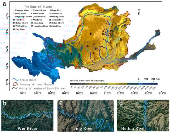
There is a long history of the formation of the Yellow River, but the Yellow River does not follow the shortest path into the sea, so do its tributaries, which indicates that their developing processes are mainly controlled by geological tectonic movement. According to the division of Yuan et al. [28], the Loess Plateau can be divided into Ordos stable platform, Longxi area, and Fenwei Cenozoic Rift, as shown in Figure 1.

Ordos platform is the earliest continental core of the Chinese mainland and a stable small uplift area of Cenozoic. In the late Pliocene, the Ordos platform was uplifted as a whole, and the river erosion was strong. The river undercut bedrock river about 80–100 m, and the Neogene red soil accumulation was also cut and eroded, resulting in the pre-Quaternary paleo-topography. The present loess landform basically inherits the ancient landform before the Quaternary, but the later erosion makes the loess landform more complex and broken. After entering the Quaternary, erosion is still ongoing [28].

For Fenwei Cenozoic Rift Valley, it is a very special tectonic unit in the southeast of Loess Plateau [28]. Since Eocene, Fenwei Rift has been under the action of the extensional stress field. The extensional stress perpendicular to the longitudinal axis of the rift has become the basic driving force for the development of Fenwei Rift and the Neotectonic movement. The subsidence of the basin is accompanied by the rise of mountains on both sides of the rift and platforms on both sides of the river. The Loess landforms in this area are mainly loess tableland landforms. Quaternary Aeolian Loess is deposited on the platform composed of fluvial and lacustrine deposits in the rift valley, with a double-layer structure. The lower part is fluvial and lacustrine deposit, the upper part is Quaternary Aeolian Loess, and the top surface is flat. Because the basin is narrow, there are few large tributaries and the downcutting of the tableland is not strong [54].

In terms of the effect of the climate on the sediment discharge, we choose the Jing River Basin as example to reveal the change in sediment yield. Zhang et al. [55] suggested that water diversion works, soil and water-conservation measures, and variations in rainfall are the major contribution to the changes in sediment discharge. In the Jing River Basin, the average annual rainfall for the period from 1956–1969 was 534.6 mm, and from 1970–1979, 1980–1989, 1990–1999, and 2000–2015, it was 490.2 mm, 491.4 mm, 474.2 mm, and 522.2 mm. While the average annual rainfall from 1990–1999 decreased by 3.5% compared to 1980–1989, the sediment discharge increased by 28%. Therefore, Zhang et al. [55] pointed that in the Jing River Basin, the effect on sediment yield cannot be attributed to the average annual rainfall, and they concluded that despite the increase in annual rainfall, heavy rainfall has experienced a significant decrease, which greatly affects the sediment yield.

Climate change may lead to more frequent extreme weather events in the future, suggesting that heavy rainfall is likely to increase in the Yellow River Basin and result in higher sediment discharge. Therefore, Zhang et al. [55] suggested that the construction of the Dongzhuang Reservoir on the Jing River and the Guxian Reservoir in the middle reaches of the Yellow River should remain an essential consideration in the river’s runoff and sediment management system. Our study shows that the sinuosity of constrained rivers on the Loess Plateau is generally low, but there are still highly sinuous bends. The development of these bends is limited by the mountains on both sides, indicating that deposition is more pronounced than erosion when these rivers are within the influence range of a reservoir. The planform characteristics of the rivers studied provide some support for selecting reservoir sites and arranging dredging projects after reservoir construction. To enhance sediment flushing after reservoir construction, it is advisable to avoid areas with highly sinuous bends and tributary confluences, where complex hydrodynamic conditions may reduce the effectiveness of sediment discharge.