Moving Target Geolocation and Trajectory Prediction Using a Fixed-Wing UAV in Cluttered Environments

1. Introduction

There are a wide range of application scenarios for UAVs to track moving targets, such as fire strikes against hostile targets in the military field [1] and wildlife surveillance in the civilian field [2]. In these mission scenarios, the random and highly dynamic motion of the target poses a huge challenge to a fixed-wing UAV in tracking the target [3]. The high dynamic motion of fixed-wing UAVs may cause targets to appear and be lost frequently in the field of view. At the same time, environmental factors, such as illumination [4] and occlusions [5], as well as factors such as changes in the scale of the target and random motion [6], all pose challenges to drone tracking of targets.

The scenario of a fixed-wing UAV tracking a moving ground target can be simplified into a model of the UAV (or camera) motion and the target’s motion, since the camera is mounted on a fixed-wing UAV [7]. Due to the high-speed motion of the camera and the motion of the target, the relative motion between the two is more complicated, which adds more uncertainty to the state of the target estimated by the UAV [8]. In addition, affected by load and power consumption, the computing resources of the UAV’s onboard processor are limited [9]. The rapid relative motion between the UAV and the target places high demands on the real-time performance of the system. With a delay of only a few milliseconds, the information received by the ground station will be very different from the current real state of the target [10]. Therefore, the real-time performance of the method proposed is an important factor that cannot be ignored.

Some works have focused on vision-based UAV tracking and localizing of ground targets [11,12,13]. Hong et al. [14] adopted the detection-tracking mode and improved a target tracker named DeepSORT by optimizing the network structure of the target detector Yolo4. Micheal et al. [15] used a deeply supervised object detector (DSOD) for the detection, and then improved its tracking capability by using a Long–Short-Term Memory (LSTM) to track the target of the detection. Eckenhoff et al. [16] proposed a tightly-coupled visual inertial localization and 3D rigid-body target tracking method and constructed a visual–inertial navigation system (VINS) framework based on a multi-state constrained Kalman filter. Instead of considering the target as a moving mass point, the authors used a dynamic 3D rigid-body model to estimate the position, direction, and velocity of the target and provided an observability analysis with geometric interpretation. In [17], the authors studied the multiple rigid body localization problem, proposed a cooperative approach using sensor–anchor and sensor–sensor measurements, and developed a cooperative semidefinite programming (CSDP) solution for jointly estimating the positions and orientations of multiple rigid bodies.

Thomas et al. [18] used a single onboard camera and an inertial measurement unit to estimate the relative position of a spherical target. They considered fitting a cone to a set of 3D points, which is resilient to partial occlusions. Zhang et al. [11], combining monocular aerial image sequences and GPS data, proposed a fast and accurate multi-target geolocation algorithm based on 3D map construction. Instead of using tightly-coupled or loosely-coupled methods, Liu et al. [19] proposed a switching-coupled backend solution method to solve the simultaneous localization and dynamic target tracking problem. Li et al. [20] developed a tracking controller for UAVs to track unknown moving targets. The relative motion between the target and the UAV was modeled in the tracking controller, and an unscented Kalman Filter and quadratic programming were combined to estimate the target state and handle occlusion. Wang et al. [21] proposed a general optimization-based visibility-aware trajectory planning method that considers the visibility of the target as a key factor in trajectory optimization, which used a continuously differentiable polynomial representation to prevent dimensionality explosion when the planning problem scales up. It jointly optimized the robot’s position and yaw angle to maximize the target visibility. Zhang et al. [13] used stereo vision technology to jointly estimate the relative altitude and yaw angle deviation between the drone and the target, a technique which can be applied to cruising and hovering flight scenarios. Algabri et al. [22] integrated a deep learning-based person-following system, using point clouds to estimate the true location of the person and online learning and prediction of the target trajectory based on the historical path of the target person. A model named AttnMove [23] was proposed based on the attention mechanism to recover individual trajectories with fine-grained resolution, and various intra-trajectory and inter-trajectory attention mechanisms were designed to address the sparsity problem.

As for the ground target trajectory recovery and prediction using flying vehicles, some works have explored the issue. In [24], the authors studied the scenario of a quadrotor UAV tracking a moving target in cluttered environments. In order to realize the online dynamic trajectory planning for a quadrotor tracking the target, the authors proposed a polynomial fitting trajectory algorithm to estimate and predict the target’s motion, and expanded the target trajectory using the Taylor formula, ignoring the high-order terms, minimizing the error between the target observation position and the Taylor polynomial expansion, and then optimizing it through the quadratic programming method. The target trajectory can be estimated and used to predict the target’s motion in a short time. Unlike their scenario, our work uses a high dynamic fixed-wing UAV instead of a quadcopter, and our tracking and trajectory recovery time exceeds 1000 s. Other studies on target trajectory prediction and recovery include trajectory prediction for multi-agent systems [25], tracking and predicting human trajectories through ground-mobile robots [26]. These studies provide good ideas for target trajectory estimation and recovery, but they are different from the trajectory estimation and recovery of moving targets based on large-scale and high dynamic scenarios in this paper.

In the previous literature, the fixed-interval smoother [27] has been used on the sparse structure of the covariance matrix to accelerate the solution of the equation through one forward recursion and one backward recursion. The Rauch–Tung–Striebel (RTS) [28] smoothing algorithm can solve the batch optimization problem efficiently and non-approximately, which uses the standard equation form of the smoothing algorithm. These algorithms need to use information from future moments to estimate the past state and cannot run online. Inspired by these methods, we propose a novel method that uses Extended Kalman Filtering [29] to geolocate moving ground targets, and then uses the optimized local weighted regression method [30] to recover the trajectory and predict the target’s motion.

This paper, based on the previous work [31], makes full use of the kinematic constraints of the moving target and uses the historical geolocation results of the target to recover the trajectory of the moving target and predict the movement of the moving target. It can effectively solve the problems of large discrete geolocation errors and easy loss of moving targets. Through real flight experiments, the algorithm proposed in this paper can be thoroughly verified.

Based on the above discussion, this paper focuses on moving ground target geolocation and trajectory recovery and estimation using a fixed-wing UAV. The main contributions of the paper are as follows.

(1): A vision-based UAV geolocation and trajectory recovery estimation framework for moving ground targets is proposed. This framework enables the fixed-wing UAV to stably track moving ground targets for a long time under high dynamic and speed flying conditions.
(2): Methods for online real-time recovery of moving target trajectory based on EKF geolocation and based on local weighted regression smoothing are proposed. This makes it possible to recover the historical trajectory of the target and predict the next step of the moving target.
(3): A series of real flight experiments were conducted to validate each step’s outcomes under the proposed methods, followed by comparative analysis and error assessment based on experimental results.

The organizational structure of this research paper is as follows. The first part is the introduction, which sets the stage by presenting the research motivation, significance, and a concise overview of related works. Subsequently, the second part delves into the problem formulation, which introduces system framework and model construction. In the third part, each module is introduced comprehensively, including vision-based and EKF target geolocation, trajectory recovery and optimization methods. The fourth part focuses on the real flight experiments, which serve to validate the proposed method through real experiments and conduct a comparative analysis against other relevant approaches, thereby providing a conclusive assessment of the research’s efficacy and innovation. Finally, the paper’s content is summarized in the conclusion.

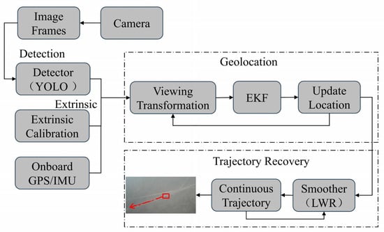
3. Proposed Method

3.1. Vision-Based Geolocation

Vision-based geolocation can be realized through camera imaging models and geometric relationships in rigid body transformations. Figure 3 is a graphical illustration of a UAV localizing ground targets.

P

is the ground target, and its imaging projection on the image is P’. The position of the ground target in the world coordinate frame can be described as follows:

$R_{P}^{(w)} = R_{c}^{(w)} + C_{c}^{w} \cdot R_{LOS}^{(c)}$

(4)

where $C_{c}^{w}$ represents the transformation matrix from coordinate system $C$ to $W$ . Through the pinhole camera model, the line of sight (LOS) direction of the target in the camera coordinate system $C$ can be obtained:

$\frac{1}{\sqrt{u^{2} + v^{2} + f^{2}}} (\begin{matrix} u \\ v \\ f \end{matrix}) = \frac{1}{|R_{LOS}|} R_{LOS}^{(c)}$

(5)

Combining Equations (4) and (5), we can obtain the following:

$(\begin{matrix} x_{c} \\ y_{c} \\ z_{c} \end{matrix}) = (\begin{matrix} x_{P} \\ y_{P} \\ z_{P} \end{matrix}) - \frac{|R_{LOS}|}{\sqrt{u^{2} + v^{2} + f^{2}}} C_{c}^{w} (\begin{matrix} u \\ v \\ f \end{matrix})$

(6)

Take the third line of Equation (6) and transpose it to get the following:

$\frac{|R_{LOS}|}{\sqrt{u^{2} + v^{2} + f^{2}}} = \frac{z_{P} - z_{c}}{(0,0, 1) C_{c}^{w} (\begin{matrix} u \\ v \\ f \end{matrix})}$

(7)

Substituting Equation (7) into the first two equations of Equation (6) yields the following:

$(\begin{matrix} x_{P} \\ y_{P} \end{matrix}) = (\begin{matrix} x_{c} \\ y_{c} \end{matrix}) + (z_{P} - z_{c}) \frac{1}{(0,0, 1) C_{c}^{w} (\begin{matrix} u \\ v \\ f \end{matrix})} [\begin{matrix} 1 & 0 & 0 \\ 0 & 1 & 0 \end{matrix}] C_{c}^{w} (\begin{matrix} u \\ v \\ f \end{matrix})$

(8)

In Equation (8), $C_{c}^{w}$ can be calculated as $C_{c}^{w} = C_{b}^{w} C_{g}^{b} C_{c}^{g}$ . The three parameters can be obtained through the camera–pod–IMU extrinsic parameters, the pod rotation angle, and the position of the drone in the world coordinate frame, respectively. The camera focal length f can be obtained through calibration, $(u, v)$ is the center of the bounding box of the target detection, and the position of the camera in the world coordinate system $(x_{c}, y_{c}, z_{c})$ can be obtained through the drone’s onboard GPS and the external parameters of the camera and autopilot. Therefore, Equation (8) is transformed into obtaining $z_{p}$ or estimating the size of $z_{p} - z_{c}$ , that is, the relative height between the camera and the target, or further, estimating the relative height between the drone and the ground target in the Z-axis direction in the world coordinate system.

Equation (8) gives a solution to the positioning of UAV-mounted targets. However, by obtaining the position of the target in the 3D world through a 2D image, only the normalized world coordinates of the target can be obtained under the condition of only two equations. Therefore, when using a monocular to locate the target, other constraints or prior information need to be added to obtain the three-dimensional coordinates of the target. The most commonly used model is the “flat ground model”, which assumes that the target moves on a flat road, or that the height fluctuation of the ground can be ignored during the movement of the target. When a small UAV performs a mission, it is assumed that the altitude of the ground target is consistent with the altitude of the UAV’s location. In this way, the relative height between the UAV and the target can be directly obtained through the onboard GPS, that is, ${h = z}_{p} - z_{c}$ , so that the position of the ground target can be directly estimated.

3.2. EKF Target Geolocation

The target’s position in the reference frame of

T

(x, y)

, and its speeds in the X-axis and Y-axis directions are

v_{x}, v_{y}

, respectively. Select the state variable of the system as

x_{k} = {(x, y, v_{x}, v_{y})}^{T}

. The geolocation result of the target through view geometry is

(\bar{x}, \bar{y})

. Over the time period Δt, assuming that the target moves in a uniform straight line and the system has no control input, the state equation of the target can be expressed as follows:

${[\begin{matrix} x \\ y \\ v_{x} \\ v_{y} \end{matrix}]}_{k} = [\begin{matrix} 1 & 0 & Δ t & 0 \\ 0 & 1 & 0 & Δ t \\ 0 & 0 & 1 & 0 \\ 0 & 0 & 0 & 1 \end{matrix}] {[\begin{matrix} x \\ y \\ v_{x} \\ v_{y} \end{matrix}]}_{k - 1} + w_{k}$

(9)

This can be shortened to the following:

$x_{k} = A x_{k - 1} + w_{k}$

(10)

where $w_{k}$ is a Gaussian white noise with mean 0 and covariance Q:

The system observation is the direct geolocation result, satisfying

z_{k} = {(\bar{x}, \bar{y})}^{T}

; then, the observation model can be written as follows:

$z_{k} = H x_{k} + v_{k} \to {[\begin{matrix} \bar{x} \\ \bar{y} \end{matrix}]}_{k} = [\begin{matrix} 1 & 0 & 0 & 0 \\ 0 & 1 & 0 & 0 \end{matrix}] [\begin{matrix} x \\ y \\ v_{x} \\ v_{y} \end{matrix}] + v_{k} = {[\begin{matrix} x \\ y \end{matrix}]}_{k} + v_{k}$

(12)

where $v_{k}$ is a Gaussian white noise with mean 0 and covariance R:

In this paper, the directly observed quantity is the center of the target in image pixel

(u, v)

, and the position of the target in the world coordinate system is

(x_{w}, y_{w}, z_{w})

. The relationship between the two can be expressed by the following function, which is denoted as

h_{k}

$[\begin{matrix} u \\ v \\ 1 \end{matrix}] = \frac{1}{z_{c}} [\begin{matrix} f_{x} & 0 & u_{0} & 0 \\ 0 & f_{y} & v_{0} & 0 \\ 0 & 0 & 1 & 0 \end{matrix}] T_{G B}^{C} T_{G F}^{G B} T_{B}^{G F} T_{V I}^{B} T_{W}^{V I} [\begin{array}{l} x_{w} \\ y_{w} \\ z_{w} \\ 1 \end{array}]$

(14)

where $z_{c} = h / c o s φ$ , $φ$ is the angle between the camera’s optical axis and the plumb direction, which can be measured by the angle of the pod and the attitude of the drone. At this point, the observation equation in the Kalman filter becomes the following:

$z_{k} = h_{k} (u_{k}, v_{k}) + v_{k}$

(15)

Taylor expansion of the function (ignoring higher-order terms above the second order) gives the following:

$z_{k} \approx h_{k} ({\bar{u}}_{k}, {\bar{v}}_{k}) + \frac{\partial h_{k} (u_{k}, v_{k})}{\partial x_{k}} |_{{\bar{x}}_{k}} (x_{k} - {\hat{x}}_{k}) + v_{k}$

(16)

The partial derivative Jacobian matrix is recorded as follows:

$H = \frac{\partial h_{k} (u_{k}, v_{k})}{\partial x_{k}} |_{{\bar{x}}_{k}}$

(17)

If the system state model is not a linear function, but a nonlinear function expressed as

f (x_{k})

, the state model can be linearized through Taylor expansion:

$\begin{array}{l} x_{k} & \approx f ({\hat{x}}_{k - 1}) + \frac{\partial f}{\partial x_{k - 1}} |_{{\hat{x}}_{k - 1}} (x_{k - 1} - {\hat{x}}_{k - 1}) + w_{k} \\ = A_{k - 1} x_{k - 1} + (f ({\hat{x}}_{k - 1}) - A_{k - 1} {\hat{x}}_{k - 1}) + w_{k} \end{array}$

(18)

The Jacobian function here is the following:

$A_{k - 1} = \frac{\partial f}{\partial x_{k - 1}} |_{{\hat{x}}_{k - 1}}$

(19)

The state error of the system is defined as follows:

$\{\begin{matrix} {\bar{e}}_{k} = {\bar{x}}_{k} - x_{k} \\ {\hat{e}}_{k} = {\hat{x}}_{k} - x_{k} \end{matrix}$

(20)

The state error transfer equation of the Extended Kalman Filter can be expressed as follows:

$\begin{array}{l} {\bar{e}}_{k} & = {\bar{x}}_{k} - x_{k} \\ \approx {\bar{x}}_{k} - (f ({\hat{x}}_{k - 1}) + A_{k - 1} (x_{k - 1} - {\hat{x}}_{k - 1}) + w_{k}) \\ = A_{k - 1} {\hat{e}}_{k - 1} - w_{k} \end{array}$

(21)

Equation (21) shows that the state error transfer equation of the system is a function related to $A_{k - 1}$ , and the system matrix $A_{k - 1}$ depends on the estimate of the current state. When the state estimate is far from the true value, $A_{k - 1}$ will also have a large deviation. The prediction update through the system matrix $A_{k - 1}$ will further amplify the error, which may eventually cause the filter to diverge.

In fact, when the observation model is linearly approximated, a similar conclusion will be drawn. This is because the EKF only linearizes ${\hat{x}}_{k - 1}$ once and calculates the posterior probability through the linear model. In fact, only high-order Taylor expansion can approximate the entire function. The first-order Taylor approximation is only valid within a very small range. Once the state model or observation model has strong nonlinearity and the working point is far away, it cannot be approximated by the first-order Taylor expansion. Therefore, the Extended Kalman Filter has high requirements for the accuracy of the initial value setting of the state, otherwise it may cause the system to diverge.

3.3. Trajectory Estimation

Traditional smoothing algorithms consider all historical data points equally, which can lead to inaccuracies, especially in dynamic environments where target motion patterns change rapidly. To mitigate this, we introduce a temporal weighting scheme that emphasizes recent data points more heavily than older ones, as shown in Figure 4. This approach ensures that the algorithm adapts swiftly to changes in target behavior, reflecting the most recent movements more accurately. Furthermore, we incorporate an anomaly detection mechanism within the LWR framework. This mechanism identifies and excludes data points that deviate significantly from the expected trajectory, thereby reducing the influence of outliers. By filtering out these anomalies, we enhance the robustness of our tracking system, ensuring that the reconstructed trajectory remains representative of the target’s actual movement.

Define weight

w_{i}

and coefficient vector

θ

. The loss function can be written as the following:

$L (θ) = \frac{1}{n} \sum_{i = 1}^{n} ω_{i} {(y_{i} - θ * x_{i})}^{2} = \frac{1}{n} ω ‖ Y - X * θ ‖^{2}$

(22)

Take the derivative of

θ

and make it equal to 0, then

θ = {(X^{T} ω X)}^{- 1} X^{T} ω Y

. Let

\hat{Y} = \hat{H} Y

, then:

$\hat{H} = {X (X^{T} ω X)}^{- 1} X^{T} ω$

(23)

In [31], we demonstrated that utilizing QR or Singular Value Decomposition (SVD) can drastically reduce the computational load associated with the LWR algorithm. By decomposing the relevant matrices into their constituent parts, we derived equation

\hat{H} = {\sqrt{ω}}^{- 1} Q Q^{T} \sqrt{ω}

, which facilitates more efficient processing without compromising accuracy.

Through experiments, it is found that in the trajectory-smoothing optimization algorithm, with the increase of data points, its error will first decrease and then increase. Therefore, too few data points are inappropriate, while too many points will lead to an increase in computing resources and memory usage. In order to prevent the weight far from the center point from fading too fast, a weight function with high power $W (x) = {(1 - {|x / d_{m a x}|}^{3})}^{3 / 2}$ is adopted, where $d_{m a x} = |x_{n} - x_{1}|$ .

Despite the advancements introduced through the refined LWR algorithm and computational optimizations, some errors in the initial trajectory estimates can still persist, particularly in scenarios with high dynamic range or noisy data. To address this, we draw inspiration from Bezier curves, a class of parametric curves widely used in computer graphics for generating smooth and predictable paths.

In our approach, we leverage the smooth predictions provided by the EKF as a basis for further trajectory refinement. By introducing control points and control lines, akin to those used in Bezier curve construction, we iteratively adjust the trajectory to better align with the expected motion patterns of the target. This process not only smooths out abrupt changes or irregularities, but also ensures that the final reconstructed trajectory is stable.

The control points serve as anchors that guide the trajectory through key positions, while the control lines define the curvature and directionality between these points. By fine-tuning the placement and influence of these control elements, we achieve a balance between fidelity to the original data and smoothness in the reconstructed trajectory. The proposed algorithm is shown as Algorithm 1.

Algorithm 1. Trajectory recovery and optimization

1: Input: EKF solution results

x

, number of samples

n

, weighting function

W (x)

.
2: Output: recoverd and optimized trajectory
3: Initialize the number of samples

n

, and EKF solution results

x_{n}

4: for

i

← 1 to

n

do
5: eliminate outiers

x_{i}

based on

3 σ

method
6: end for
7: While tracking task not finished
8: calculate the step distance

d

between each sample and the current time
9: calculate the weight

ω

corresponding to each sample
10: perform QR or SVD decomposition on the weighted sample to obtain

Q

11: solve the locally weighted regression solution to obtain the coefficient

θ

12: calculate the data smoothing result at the current time
13: optimize smoothing results
14: End While

4. Flight Experiment and Discussion

4.1. Experimental Environment

As shown in Figure 5b, the experiment was carried out in an open outdoor area with relatively flat terrain and minimal obstructions. This area provided sufficient space for the UAV to maneuver and for the moving ground target to travel. The geographical location was carefully chosen to ensure stable GPS signals for both the UAV and the target, which is crucial for accurate positioning and tracking. The weather conditions during the tests were also taken into account. Fair weather with mild wind speeds was preferred to minimize the impact of external factors on the flight performance of the UAV and the movement of the ground target. Wind speeds remained within a range that allowed the UAV to maintain stable flight and accurate tracking.

The UAV flight platform (Figure 5c) was a fixed-wing model equipped with a multisensor suite for autonomous navigation and target tracking. The visual system comprised a forward-facing RGB camera (resolution: 1280 × 720 pixels, frame rate: 30 Hz, focal length: 3.6 mm) mounted on a two-axis gimbal for image stabilization. Navigation data were acquired via a Pixhawk 4 autopilot integrating a GPS module and an IMU. The onboard processor in the UAV is Odroid-xu4. These subsystems enabled real-time fusion of geospatial positioning, inertial dynamics, and visual data for trajectory estimation. The moving ground target was a vehicle (Figure 5d) that was equipped with a GPS tracker to record its moving position, so as to make a comparison with the position prediction and trajectory recovery methods proposed in this study. The target was designed to move at various speeds and follow different trajectories to simulate real-world scenarios of moving objects on the ground.

During the experiment, the UAV maintained an altitude ranging from 60 to 80 m as shown in Figure 5a. This height was chosen to balance the need for a clear view of the ground target and to stay within the operational limits and safety regulations. The flight path of the UAV was designed to cover a significant portion of the experimental field, allowing for comprehensive tracking of the target. The entire tracking process lasted over 1000 s, during which the UAV continuously adjusted its position and orientation based on the real-time pixel position of the target detected in the camera.

4.2. Target Tracking

Figure 6 shows the tracking and positioning process of the experimental scenario described above. Processes A-E represent the five stages of the drone starting to search for the target, the drone stably tracking the target, the first big turn of the ground target, the second big turn of the ground target, and the end of tracking. The positioning results of the entire process are represented by red dots. In the initial stage of tracking, the drone searches for the ground target, and the target position estimation results are distributed in the area centered on the target’s true position; when the drone stably tracks the target, the positioning results fluctuate evenly around the target’s true trajectory; around the 686th second, the ground target suddenly changes its direction of movement. During this period, the target frequently enters and exits the image field of view, causing the drone and the pod to shake more, resulting in unstable positioning, and abnormal positioning values appearing at some moments; when the target turns for the second time, the positioning results gather at the corner, and instability occurs again; after the second turn until the end of tracking, the target moves in a straight line, and the drone performs stable tracking and positioning of the ground target.

When the experiment was initiated, the moving ground target was initially outside the UAV camera’s field of view. As the target started to move into the designated area, the UAV’s onboard camera systems began to search for any signs of the target. Once the target entered the camera’s field of view, the UAV’s image-processing algorithms immediately detected the presence of the object. At this moment, the UAV initiated the tracking process. It adjusted its flight path slightly to center the target within the camera frame. The UAV’s navigation system also started to record the initial position and orientation of the target relative to the UAV. This stage was crucial as it set the foundation for the subsequent tracking. The accuracy of the initial detection and the UAV’s quick response to center the target determined the success of the overall tracking experiment. If the target was not detected promptly or not centered accurately, it could lead to difficulties in maintaining a stable track during the later stages.

After the target was successfully detected and centered in the camera view, the UAV entered the stable tracking phase. In this stage, the UAV relied on a combination of its navigation and camera systems to continuously monitor the target’s position. The onboard computer processed the images from the camera in real time, extracting the precise pixel coordinates of the target. These pixel coordinates were then converted into real-world coordinates using the known parameters of the camera and the UAV’s position and orientation. The UAV adjusted its flight path and speed to maintain a constant distance and angle with respect to the target. The UAV’s flight was smooth and steady, following the target’s movement with high precision.

As the tracking progressed, the moving ground target made a sharp turn. This sudden change in the target’s direction posed a significant challenge to the UAV’s tracking system. When the target initiated the turn, the UAV’s camera detected the change in the target’s movement pattern almost instantaneously. The UAV had to decelerate and change its own direction rapidly to follow the target’s sharp turn. This required a high degree of maneuverability and responsiveness from the UAV. The control systems had to adjust the angles of the UAV’s wings and the thrust of its motors precisely. During this process, there was a risk of losing track of the target if the UAV could not adjust its flight path quickly enough. So, we can see that at this stage, ground targets sometimes do not appear in the image field of view, resulting in significant positioning errors.

After the first sharp turn, the target made a second sharp turn. As with the first turn, the UAV’s camera and navigation systems worked in tandem. The camera detected the new movement of the target, and the navigation system calculated the necessary adjustments. However, this time, the UAV had to consider its own position and velocity after the first turn. It had to make more complex calculations to determine the optimal flight path to resume tracking. The UAV might have deviated slightly from the ideal tracking path due to the first turn, and now it had to correct these errors while following the target’s new turn. The UAV adjusted its yaw, pitch, and roll angles more precisely to align itself with the target’s new trajectory. Despite the challenges, the UAV managed to maintain tracking, although the accuracy might have been slightly affected compared to the stable tracking stage. This stage demonstrated the UAV’s ability to handle consecutive and rapid changes in the target’s movement, which is essential in real-world applications where targets may exhibit unpredictable behavior.

After a certain period of tracking and following the target’s various movements, the tracking experiment came to an end. At this point, the UAV ceased its active tracking and started to return to a designated landing area. The data collected during the entire tracking process, including the UAV’s flight path, the target’s position at each time step, and any relevant sensor readings, were stored for further analysis. The end of the tracking experiment also provided an opportunity to assess the overall reliability and robustness of the UAV and its associated systems.

To analyze the errors in the process of a drone tracking a moving ground target, an experiment was conducted; the results are shown in Figure 7.

Figure 7a shows that there were outliers with extremely large positioning errors. These outliers mainly stemmed from the loss of the target from the image field of view. When the drone fails to detect and track the target accurately in the image, the positioning algorithm may generate incorrect position estimations, leading to significant deviations in the positioning results. This could be due to various factors such as rapid changes in the target’s motion pattern, or unfavorable environmental conditions that affect the visibility and detectability of the target.

Figure 7b shows that the error exhibited a sinusoidal periodic variation. The primary causes of this periodicity were sensor noise and mechanical installation errors. Sensor noise, which is inherent in the measurement process, can introduce random fluctuations in the position data. Additionally, mechanical installation errors, such as misalignments or vibrations in the sensor mounting, can cause systematic variations in the measured values. These combined effects result in the observed sinusoidal pattern of the error over time.

To solve the problem of outliers, some strategies and algorithms could be adopted for improvement. For example, removing outliers that result in significant positioning errors due to target loss can improve the accuracy of target localization. In order to reduce the impact of sensor noise and mechanical installation errors, the system deviation should be optimized through external parameter calibration. In addition, Kalman Filtering can be used to reduce the impact of noise and more accurately estimate the true target position.

4.3. Trajectory Recovery

In the pursuit of accurate tracking and trajectory recovery of moving ground targets using a fixed-wing UAV, a series of experiments were conducted. The core objective was to develop and evaluate a comprehensive framework that combines multiple algorithms and optimization techniques. The experimental results are presented through four result graphs, as shown in Figure 8a–d, each representing a successive stage of refinement in the target positioning and trajectory estimation process. Table 1 presents the process of algorithmic improvement by summarizing the MAE (Mean Absolute Error) values of each method. These graphs not only showcase the performance of individual algorithms but also highlight the cumulative improvements achieved through the integration of different techniques.

As shown in Figure 8a, the EKF’s first step in prediction is an essential initial attempt to estimate the target’s position. However, it shows significant differences when contrasted with the ground truth. This deviation can be attributed to several factors. The model used in the prediction might oversimplify the real-world target motion, failing to account for various uncertainties and disturbances. Sensor inaccuracies also play a major role. The data obtained from onboard sensors of the UAV, such as GPS and IMU, inherently possess errors, which are then incorporated into the prediction, leading to inaccuracies.

In the second step, EKF update aims to correct predictions based on new sensor measurements. Although it did improve the results to some extent, the updated position still does not fully reflect the actual situation. The main reason is that the target is lost from the field of view, resulting in outliers that affect the EKF results.

After the outlier rejection and optimization, a notable improvement is observed. Outliers, which could be caused by sensor malfunctions or momentary occlusions, are identified and removed. This step significantly reduces the impact of spurious data, making the optimized result much closer to the ground truth. It demonstrates the importance of robust data preprocessing in enhancing the overall accuracy of target positioning.

Figure 8b presents the solution results of the EKF. After obtaining the positioning results from the EKF, we apply the LWR algorithm to estimate the target’s trajectory. The EKF generates a series of discrete position points over time, while the LWR aims to fit a smooth curve through these points to depict the target’s path. However, the resulting trajectory deviates from the true one. This is because the residual errors from the EKF, which are not entirely eradicated, influence the trajectory estimation. These errors can cause the estimated trajectory to deviate in terms of curvature and overall shape. Additionally, the LWR algorithm has its own limitations. It assumes a certain level of local smoothness in the data, which may not be valid for all target motion patterns. For instance, if the target makes rapid or irregular maneuvers, the algorithm may have difficulty accurately capturing the changes, leading to disparities between the estimated and true trajectories. In terms of accuracy, for the EKF alone method, the MAE values in the X and Y directions are 9.67 m and 9.16 m, respectively. When using the EKF + LWR method, the accuracy is improved by 16.1% in the X direction and 7.8% in the Y direction. This improvement demonstrates the effectiveness of combining the EKF with the LWR algorithm in enhancing the accuracy of target trajectory estimation.

After optimizing the integrated EKF + LWR + Bezier framework, the estimated trajectory demonstrates significant improvement, with quantitative evaluations showing 41.4% and 14.5% reduction in X and Y direction errors, respectively, compared to EKF alone, and 31.9% and 7.3% improvement over the EKF + LWR baseline. These enhancements are achieved through three key optimizations: (1) refining the LWR weighting function to dynamically balance measurement reliability and temporal proximity, effectively suppressing noise while preserving motion details; (2) expanding the regression sample size to 121 points to enhance accuracy without sacrificing efficiency—extensive trials confirm the trajectory smoothing computation time remains below 20 ms on the embedded Odroid-XU4 platform; (3) incorporating physical motion constraints via third-degree Bezier curves, ensuring kinematically feasible trajectory estimates.

The final step of using the Bezier curve-inspired method for optimization yields the most accurate estimation trajectory. This method can effectively interpolate between the optimized local weighted regression results, creating a continuous and visually appealing trajectory. The 3rd-degree Bezier curve was selected to balance smoothness and computational efficiency. By adjusting the control points based on the characteristics of the target’s motion and the desired level of accuracy, the final trajectory closely follows the true trajectory. This final optimization step not only improves the visual match between the predicted and true trajectories but also enhances the overall quality of the trajectory estimation.

5. Conclusions

This work has presented a comprehensive approach for drone tracking of moving ground targets and the recovery of their motion trajectories. The utilization of the EKF algorithm for target positioning has laid a solid foundation. Despite its effectiveness, the EKF has shown certain limitations due to factors such as sensor inaccuracies and the inability to fully account for complex real-world target behaviors. However, through a series of optimization strategies, the performance has been enhanced.

The incorporation of the local weighted regression algorithm for online real-time trajectory smoothing has significantly contributed to obtaining more continuous and reliable trajectory estimations. It has mitigated the impact of noise and fluctuations in the positioning data. Yet, it also has its own drawbacks, especially in handling sudden and drastic changes in the target’s motion.

The optimization algorithms applied to both the positioning and trajectory smoothing processes have proven crucial. They have effectively addressed issues like outlier rejection, which has reduced the influence of spurious data on the overall results. Through these optimizations, the accuracy of the target positioning and the resemblance of the estimated trajectory to the ground truth have been substantially improved.

Future research directions could focus on further refining the EKF model to better adapt to highly dynamic and unpredictable target motions. Additionally, exploring more advanced sensor fusion techniques to enhance the quality of input data for the algorithms is warranted. The improvement of the local weighted regression algorithm or the exploration of alternative trajectory smoothing methods that can handle abrupt changes more precisely is also essential. Overall, this study serves as a significant step forward in the field of drone-based target tracking and trajectory recovery, but continuous efforts are required to achieve even higher levels of accuracy and reliability for a wider range of practical applications.

Source link

Yong Zhou www.mdpi.com

Greenberg News

Moving Target Geolocation and Trajectory Prediction Using a Fixed-Wing UAV in Cluttered Environments

1. Introduction

3. Proposed Method

3.1. Vision-Based Geolocation

3.2. EKF Target Geolocation

3.3. Trajectory Estimation

4. Flight Experiment and Discussion

4.1. Experimental Environment

4.2. Target Tracking

4.3. Trajectory Recovery

5. Conclusions

Greenberg

1. Introduction

3. Proposed Method

3.1. Vision-Based Geolocation

3.2. EKF Target Geolocation

3.3. Trajectory Estimation

4. Flight Experiment and Discussion

4.1. Experimental Environment

4.2. Target Tracking

4.3. Trajectory Recovery

5. Conclusions

Related Posts

Properties of a Static Dipolar Impurity in a 2D Dipolar BEC

Sharing Price Announcements

Influence of Malted Chickpea on the Composition of Volatiles in Hummus

Greenberg