Operating Point Optimization of Agricultural Tractor–Implement Combinations as Constraint Optimization Problem

1. Introduction

In agriculture, tractors are primarily used as a power source, whether in the form of drawbar pull, via the PTO shaft, or hydraulically [1]. Nowadays, efficiency optimization in agriculture is usually limited to the tractor’s drivetrain in order to provide the power required for the work process as efficiently as possible. Standardized performance requirements, such as the DLG PowerMix [2], are used to evaluate the efficiency of tractors. However, the efficiency improvements in this context are limited to improving the physical machine setup and the behavior regarding a specified control input.

Alternatively, the efficiency of the work process, e.g., tillage, can be optimized by adapting the control inputs during the actual task. This increases the optimization potential but results in a complex optimization problem since, in addition to the tractor’s drive train, the characteristics of the implement need to be taken into account. Likewise, the agronomical requirements are crucial, as efficiency optimization must not be achieved at the expense of the yield. Holistic optimization of agronomical work processes must set the yield in relation to the effort required, i.e., costs or fuel consumption.

Renius described the variety of potential objectives that can be optimized during fieldwork as speed, process quality, energy consumption, safety, environmental protection, comfort, and total production costs [3]. As the yield depends on many factors and is not observable during soil cultivation, process quality is used as a substitute to take the agronomical requirements into account.

In recent years, research has focused on individually describing and optimizing some of these target criteria. For example, approaches to observe the process quality using camera-based or lidar-based approaches have been presented in [4,5,6,7]. In [8,9], the authors focused on optimizing machines’ performance and energy consumption.

In both cases, the research focused on one optimization target, neglecting the others. However, combining these separate objectives poses a major challenge to the automation of the whole task.

Steinhaus presented an approach to combine the objectives of process quality and efficiency into one unified target function to be able to evaluate the individual processing steps in the process chain [10].

Boysen et al. used a deep learning approach to predict the result from adaptation of control inputs to process quality parameters and machine-internal parameters, which could potentially also be used for state optimization [11].

In previous work, we proposed an approach to combine the objectives of process quality and energy efficiency using constraints for either process efficiency or process quality, respectively, using the example of agricultural tillage. The target was to use this approach to optimize the state of the machine combination [12].

Thus far, to the best of our knowledge, no holistic approach has been developed to optimize soil cultivation. This paper aims to address this research gap by presenting an approach to optimizing tillage with respect to agronomical requirements. The approach includes the tractor’s characteristics, the influence of the implement, and the agronomical requirements of the soil cultivation task and provides multiple possible objective functions depending on whether to optimize overall costs, efficiency, or process time.

The paper is structured as follows: In Section 2, the theoretic considerations leading to the constraint optimization problem for the holistic optimization of the cultivation task are derived. In addition, the representation of the state of a tractor–implement combination is described. Next, in Section 3, the experimental setup is explained that illustrates the approach in the case of soil tillage with a cultivator. In Section 4, the results of the soil tillage process are presented. The advantages and limitations of the presented approach are discussed in Section 5 before Section 6 concludes the paper.

2. Materials and Methods

It is assumed that all parameters required to describe the state of a machine combination can be combined in a single state vector

\vec{x}

. A general state description for tractor implement combinations is possible by splitting the state vector into control parameters

\vec{w}

, interface parameters

\vec{τ}

, and internal parameters

\vec{θ}

$\vec{x} = [\vec{w}, \vec{τ}, \vec{θ}]$

(1)

The control vector $\vec{w}$ describes adjustable parameters like operating speed, rotatory speeds of power take-offs, hydraulic volume flows, and electric flow. For agricultural machinery, the combination of the tractor with various implements features a unique adaptability, and the power demand of the process is heavily impacted by the choice of implement. Therefore, it is advantageous to separate the interface parameters $\vec{τ}$ , which describe the interactions at the connecting point between the tractor and the implement. The commonly available interfaces can transmit forces, torques, fluid pressures, and voltages. The state vector is completed with the tractor’s internal parameters $\vec{θ}$ , like the fuel rate and engine torque. These parameters are not adjusted directly for optimization but result from the combination of the other parameters.

Given an objective function

h (\vec{x})

, an optimization of the machine state using the control parameters

\vec{w}

can be described as follows:

$\underset{\vec{w}}{arg max} h (\vec{x})$

(2)

The universal optimization objective in agricultural field work can be described as maximizing the harvest yield related to the required resources. These resources can include energy input, monetary values, or production time.

$h (\vec{x}) = \frac{Harvest Yield}{Resource Input}$

(3)

This general process objective has the issue that the harvest yield is not only impacted by the process quality of each specific task within the agricultural production chain but also depends on the type of plant that is cultivated, the composition of the soil, and the effects influenced by weather, such as the moisture of the soil.

While research has already been conducted to describe the process quality of specific tasks, the relationship between the process quality of every single step in the agricultural production chain and the harvest yield is not yet quantifiable for every step.

This leads to the issue that the objective function $h (\vec{x})$ is not observable during machine operation. Standard optimization techniques like Pareto front optimization can, therefore, not be deployed since the optimization requires measurability of the objective function.

However, a human operator can use their experience to define process parameters that are supposed to have the best impact on the harvest yield. In consequence, the objective function $h (\vec{x})$ can be optimized by minimizing the resource input as long as this optimization occurs within the specified boundary conditions.

Constraints can be any given function of the state vector. Mathematically, this optimization problem and the proposed constraints are as follows [13]:

$\begin{matrix} maximize & h (\vec{x}) \\ by varying & \vec{x} \\ subject to & c_{i} (\vec{x}) = 0 & for i = 1, \dots, n \\ c_{j} (\vec{x}) \geq 0 & for j = 1, \dots, m \end{matrix}$

(4)

These constraints can take multiple forms and can vary between specific tasks in the production chain.

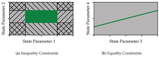
One option is the introduction of equality constraints $c_{i} (\vec{x})$ , where a specific combination of state parameters must permanently be satisfied. An example of equality constraints could be the specification of a relatively shallow working depth for stubble cultivation, in contrast to a high working depth for primary tillage. Another option is restricting the optimization space by introducing inequality constraints $c_{j} (\vec{x})$ . These constraints determine that specific state parameters or parameter combinations must be within a specified optimization scope. Typical inequality constraints are, for example, speed limitations (minimum/maximum) during tillage operations. This ensures the functionality of the implement and, consequently, the effective execution of the process.

The two options are visualized in Figure 1 in a simplified manner by constraints between two of the parameters of the state vector.

As the defined restrictions ensure the correct execution of the process, influences on the variation in the operating point in the defined limit ranges are regarded as constant with regard to the resulting harvest yield.

h (\vec{x})

can be expressed as a specific, observable target function

h^{*} (\vec{x})

multiplied by the constant, non-observable part c, which considers the effect on the harvest yield:

$h (\vec{x}) = h^{*} (\vec{x}) \cdot c$

(5)

Observable target functions, such as the productivity functions proposed by Scherer [14], can be adapted to agricultural field work. These functions facilitate the quantification of specific performance metrics.

The productivity concerning time, expressed in hectares per hour (ha/h), represents the processed field area and is determined by the operating speed v and the working width d:

$h_{time}^{*} (\vec{x}) = v \cdot d$

(6)

Energy productivity, often referred to as energy efficiency, is expressed in hectares per liter (ha/L). This metric is calculated by relating the processed field area to the fuel consumption rate B:

$h_{energy}^{*} (\vec{x}) = \frac{v \cdot d}{B}$

(7)

Monetary productivity, expressed in hectares per euro (ha/€), incorporates fuel costs, machine rental costs, and labor wages. The parameters include

C_{fuel}

, representing the fuel price per liter;

C_{area}

, which quantifies the machine costs per unit of processed area (commonly applied in implement rentals [15]); and

C_{time}

, denoting the cost per hour for tractor rental and operator wages [15].

$h_{money}^{*} (\vec{x}) = \frac{v \cdot d}{C_{fuel} \cdot B + C_{area} \cdot v \cdot d + C_{time}}$

(8)

Each of these objective functions depends on parameters derived from the machine state vector $\vec{x}$ , as previously introduced, and can be used as an optimization basis.

Despite the fact that the current status of the machine combination can be observed in principle by measuring the parameters contained in the state vector $\vec{x}$ , optimization by means of iterative adjustment of the machine status within the specified process limits would influence the processing quality. If environmental variables are changed, subsequent iteration loops are required to find the new optimum point, which makes continuous operation at the optimum operating point more difficult. A much more convenient optimization variant opens up if the possible state space of the machine combination can be modeled directly using the measurement of a single operating point as input for a prediction model. This approach avoids the otherwise necessary optimization iterations, as these can now be carried out in the model and no longer require any physical adjustments.

Various influences must be considered to predict the parameters that describe the state of the machine combination. The machine state is influenced by the environment in which the current process is carried out—for example, the type of soil and the slope. Furthermore, process parameters introduced by the tractor–implement constellation and settings, together with the defined process constraints, have an impact on the state. The last influence to consider is the effect of control inputs. Therefore, we define the control vector, which is a subset of the state vector with parameters that can be adapted independently. The predicted state

\hat{\vec{x}}

can, therefore, be expressed as a function of the environment parameters

\vec{ϵ}

, the process parameters and constraints

\vec{p}

, and the control parameters

\vec{w}

$\hat{\vec{x}} = f (\vec{ϵ}, \vec{p}, \vec{w})$

(9)

The machine state prediction process is structured similarly to the power flow of the process coming from the control input, the resulting power demand of the process, and the respective internal drivetrain parameters required to provide the requested power. At each step, all essential parameters for the description of the machine state are selected to be included in the state vector. Each component of the prediction architecture must thereby consider the current environment and the given process parameters. The prediction approach is visualized in Figure 2.

In the first step, control parameters are specified to define the operating point. The process’s power requirement is then determined on this basis. This is accomplished separately for each mounted implement, taking into account the relevant environmental parameters and process parameters so that, ultimately, the power requirement resulting from the process at the interfaces between the implements and the tractor is known. This power requirement is then used to calculate the tractor’s internal operating point, again taking into account the environment and the process conditions. This allows the consideration of losses that occur in the drivetrain. The result is the previously introduced uniform description of the machine state, which contains the control input, the load at the interfaces, and tractor-internal parameters.

3. Experiments

The method was applied during maize stubble cultivation on a field located near Osterzell, Germany, on one day in October 2024 without precipitation. The field exhibited a constant slope between minus two and plus two degrees, depending on the driving direction. The soil type of the field was classified as loamy. Although the soil was moist, it was passable and workable, with no negative impact on the soil structure. Detailed soil type and soil moisture measurements were not conducted. The tractor used for the experiment was a Fendt 724, while the tillage implement was a LEMKEN Karat 10 KUTA with a width of 4 m. The ballasting was performed using a front weight of 1250 kg. The machine combination is shown in Figure 3.

In accordance with the presented approach, to assure the process quality, a working depth condition, and a speed boundary condition were set. The process quality of this task depends heavily on the choice of working depth t and, therefore, varies between different possible applications of a cultivator during the production chain. In line with [16], the operator begins with the shallowest depth possible to minimize energy requirements. Subsequently, the depth is adjusted incrementally downward until a satisfactory work result is achieved. The best working depth for stubble cultivation depends on the amount of organic material on the surface and the site conditions—common are working depths of up to 20 cm [16]. For the given field, the human operator judged the work result satisfactory at a depth of

t = 17

cm, which was fixed as an equality constraint for the subsequent experiment.

Furthermore, during the reference passes, an issue with inadequate surface smoothing at very low speeds was observed by the operator. This speed constraint was set as a boundary constraint, since no negative impact of high speeds was observed.

The maximization of the productivity concerning energy usage for the task (Equation (7)) was selected as the optimization objective. As control input, the adaption of the speed of the machine combination was chosen.

For the state description and prediction, the model was reduced to the forces acting in the direction of travel (parallel to the ground), while the acceleration forces were neglected. All required sensor signals were collected from the standard CAN-BUS and processed using a moving mean filter with a window size of 1 s.

A weight was attached to the tractor’s front interface to improve the machine combination’s traction characteristics. The weight with a fixed mass m requires propelling forces

F_{x, w e i g h t}

depending on the gravitational acceleration g when driving on a slope

δ

$F_{x, w e i g h t} = m \cdot g \cdot s i n (δ)$

(13)

According to the presented method, these characteristics can be described as the influence of the environment

\vec{ϵ}

, the influence of the process

\vec{p}

, and the influence of the control input

\vec{w}

. The gravitational acceleration and the slope of the field are parameters that depend on the environment and cannot be adapted, as it is assumed that the navigation and choice of path are determined in advance and cannot be optimized. The mass of the implement is a process-specific constant since the weight can be adjusted in advance to optimize the weight distribution, but is not adaptable during operation.

${\vec{ϵ}}_{w e i g h t} = (\begin{matrix} g \\ δ \end{matrix}), {\vec{p}}_{w e i g h t} = (\begin{matrix} m \end{matrix}), {\hat{\vec{τ}}}_{w e i g h t} = (\begin{matrix} F_{x, w e i g h t} \end{matrix})$

(14)

The cultivator at the rear interface of the tractor requires draft forces to operate. The load due to the soil moving was specified according to ASAE D497.7 [17]. On the one hand, the overall power requirement is caused by this movement of the soil due to the process itself, but also by the force of gravity when driving on slopes.

$F_{x, c u l t i v a t o r} = s_{D} \cdot d \cdot t \cdot (46 + 2.8 \cdot v) + m \cdot g \cdot s i n (δ)$

(15)

The parameters can be assigned to the respective vector accordingly.

${\vec{ϵ}}_{c u l t i v a t o r} = (\begin{matrix} g \\ δ \\ s_{D} \end{matrix}), {\vec{p}}_{c u l t i v a t o r} = (\begin{matrix} m \\ d \\ t \end{matrix}), {\hat{\vec{τ}}}_{c u l t i v a t o r} = (\begin{matrix} F_{x, c u l t i v a t o r} \end{matrix})$

(16)

In the practical application, the parameters

s_{D}, w,

and t are combined into a single parameter calculated from the machine’s current operating point, as in [9].

The interface state vector combines the load demand of the implements mounted at the front or the rear as

$\hat{\vec{τ}} = [{\hat{\vec{τ}}}_{f r o n t}, {\hat{\vec{τ}}}_{r e a r}] = (\begin{matrix} F_{x, f r o n t} \\ F_{x, r e a r} \end{matrix}) = (\begin{matrix} F_{x, w e i g h t} \\ F_{x, c u l t i v a t o r} \end{matrix})$

(17)

For the specified objective function, only knowledge of the fuel rate is required. Therefore, all internal state parameters except for the fuel rate are omitted.

An artificial neural network was used to predict the internal state of the tractor, taking the control vector and the state of the tractor–implement interfaces as prediction inputs. Furthermore, to include environmental effects in the prediction model, the slope and an assumption regarding the machine’s traction characteristics are part of the network’s input vector. In previous experiments, it was determined that the calculated slip values based on the provided internal signals of the tractor are subject to very high noise. As a result, the use of complex slip models based on this inaccuracy of the current machine state leads to strong oscillations in the prediction model during optimization. Therefore, the assumption of constant slip was used in the tests, which is associated with strongly increasing inaccuracies with increasing speed differences between the predicted state and the current state. However, this approach leads to a more stable behavior of the optimizer and to better prediction results than the complete exclusion of the traction characteristics from the input of the network.

For practical reasons, the input of the neural network regarding the slip was not the slip rate s itself but rather the respective theoretical speed

v_{t h e o}

of the tire and the given speed from the control vector.

$v_{t h e o} = \frac{v}{1 - s}$

(19)

This allows the direct setting of this parameter as the new target speed of the tractor since the cruise control uses the theoretical speed as a reference.

${\vec{ϵ}}_{t r a c t o r} = (\begin{matrix} δ \\ v_{t h e o} \end{matrix}), {\vec{p}}_{t r a c t o r} = (), \hat{\vec{τ}} = (\begin{matrix} F_{x, f r o n t} \\ F_{x, r e a r} \end{matrix}), \hat{\vec{θ}} = (\begin{matrix} B \end{matrix})$

(20)

The training dataset for the neural network contained 101,440 operating points collected from previous tillage experiments conducted with a cultivator. Each data point consisted of the parameters listed in ${\vec{ϵ}}_{t r a c t o r}, {\vec{p}}_{t r a c t o r}, \vec{w}, \vec{τ}$ as inputs and $\vec{θ}$ as the output. The recorded and synchronized sensor signals were standardized by subtracting the mean and scaling to unit variance using PyTorch’s StandardScaler.

The neural network was implemented in PyTorch and trained to minimize the mean absolute prediction error of $\hat{\vec{θ}}$ .

For the training process, the Adam optimizer with a batch size of 512 was used, and a hyperparameter search was conducted using Bayesian optimization to optimize other architecture parameters. The discrete hyperparameter space is described in Table 1. To ensure the model’s applicability, five-fold cross-validation was performed during the hyperparameter search in combination with early stopping (patience = 5).

The final architecture of the neural network consisted of a fully connected network with three layers of 128 neurons each.

As an optimization scheme, the presented state prediction scheme was applied once every second in the constrained optimization space of 4 km/h

\leq v \leq

20 km/h in discrete steps of 0.5 km/h to make sure that the minimum speed did not exceed the provided boundary condition and that the maximum speed that was evaluated exceeded the maximum power output of the tractor. The predicted states were evaluated using the overall energy efficiency (Equation (7)) as the objective function, and the best state was selected as the new control target of the tractor if the expected outcome of the state transition would lead to an increase of a minimum of 5% of the objective function. This was implemented to avoid unnecessary oscillations due to relatively small changes in the objective function within the optimization space.

4. Results

In the following, the mean fuel efficiency is compared to parallel rows on the same field. For the reference rows without optimization, the speed is set to 5 km/h, 7.5 km/h, and 10 km/h using the cruise control. The actual speed of the machine is lower than the theoretical speed of the cruise control due to wheel slip. Table 2 lists the mean speed, the mean efficiency, and the relative efficiency improvement compared to a reference speed of 7.5 km/h for the downhill pass (negative slope).

In the downhill pass, the algorithm improved energy efficiency by 5.9% compared to a constant theoretical speed of 7.5 km/h (6.69 km/h with wheel slip). Reducing the theoretical speed to a lower constant speed of 5.0 km/h (4.55 km/h with wheel slip) improves efficiency by 4.7%. However, compared to the algorithm, the improvement is lower at a much higher speed reduction. In direct comparison with the full-throttle pass, the algorithm achieved an efficiency improvement of 23.3%.

A pass in the uphill direction was conducted with the identical setup to change the influence environment and, thereby, also the optimal operating point. These results are visualized in Table 3.

For the uphill pass, an improvement of 6.3% compared to a constant theoretic speed of 7.5 km/h (6.45 km/h with wheel slip) was observed, with a lower average speed of 4.99 km/h compared to the uphill pass.

A reference speed ramp was executed parallel to the uphill pass to visualize the algorithm’s choice of operating point. The operating points chosen by the algorithm are visualized in relation to the efficiency characteristics to control variable changes. The results are presented in Figure 4.

The speed ramp demonstrates the shape of the efficiency curve without considering process quality restrictions. Therefore, it also includes unfeasible operating speeds below the minimum speed value. The figure illustrates a visual representation of the optimization process, demonstrating that the selected speed aligns with the optimal operating point of the machine combination.

5. Discussion

The analysis of the data collected in the field tests visualizes the method’s potential to optimize the machine state. The targeted operating speed of an average of 6.0 km/h was within the reference speeds of 4.55 km/h to 8.31 km/h for the downhill pass, and 4.99 km/h within 4.34 km/h and 7.67 km/h for the uphill pass, which suggests the optimization found an optimum within the scope.

The different selected operating points between the uphill and downhill passes can be explained by the additional traction force demand due to gravitational effects when driving uphill and the optimal operating point of the machine combination being set at a fixed power outcome. Henceforth, with a reduced operating speed, the required draft power is reduced to maintain the optimal operating point.

The method’s evaluation in the field showed that the general approach of predicting possible system states and comparing them with an objective function is feasible for optimizing the machine state within the constrained optimization space.

The experiments did not study whether a human operator would be able to achieve similar improvements since this depends on the operator’s experience and concentration level.

The advantage of the allocation between the prediction of the process power demand and the drivetrain characteristics is that it offers interchangeability and interoperability of the individual components of the tractor–implement combination. Furthermore, the design of the particular model components is not predetermined, allowing for allocating classical mathematical models like the model implemented to predict the cultivator’s power demand and artificial neural networks like the model for the tractor’s drivetrain behavior.

The method currently requires a manual setting of process constraints. However, with an advanced process quality measurement system, the relationship between control input and process quality might be quantifiable, and therefore, it could be used to dynamically set process constraints concerning process quality.

Improving the sensor measurements and filtering methods used to determine the machine’s current state could further improve prediction accuracy. The individual parts of the prediction algorithm can be further optimized, for example, by implementing more accurate traction models. It is to be expected that the assumption of a more complex slip model, for example, based on the relationship between tractive force and slip (e.g., [18,19,20,21]), and using assumptions for the multipass effect (e.g., [3,22,23]), should lead to improved prediction accuracy.

6. Conclusions

This paper presents a novel approach to describing the influences on machine state and defining process constraints, which allows for the systematic consideration of various process objectives. The method’s feasibility to optimize the machine state was demonstrated in field tests. Further testing is required to specify the optimization approach’s actual optimization potential and verify its functionality under different environmental conditions. Furthermore, the system’s modular usage has to be examined to allow adaptation to various implements. The required modularization and communication of the different modules must be defined to standardize the information exchange and uniformly optimize the operating point for flexible tractor–implement combinations.

Source link

Benjamin Kazenwadel www.mdpi.com

Greenberg News

Operating Point Optimization of Agricultural Tractor–Implement Combinations as Constraint Optimization Problem

1. Introduction

2. Materials and Methods

3. Experiments

4. Results

5. Discussion

6. Conclusions

Greenberg

1. Introduction

2. Materials and Methods

3. Experiments

4. Results

5. Discussion

6. Conclusions

Related Posts

Documentation on the Invasion Risk of Asclepias speciosa in Greece and Europe

Environmental Factor – May 2021: John Bucher, who studied toxic agents from A to Z, retires from NIEHS

Maui’s post-wildfire housing crisis offers a warning for Los Angeles

Greenberg