Planning Energy-Efficient Smart Industrial Spaces for Industry 4.0

1. Introduction

As the world faces increasingly intricate energy production, distribution, and consumption challenges, energy efficiency has emerged as a crucial pillar in tackling these obstacles [1]. In industrial settings, optimizing energy consumption is crucial for competitiveness and cost reduction, a challenge that industries worldwide face. For example, the industrial sector is the largest consumer of energy in Brazil [2].

Based on information from the Brazilian Energy Research Company [3], the industrial class in Brazil leads to an increase in energy consumption, with an annual rate of 3.0% in January 2025. The sector’s ongoing growth is evident in this rising pattern, while the population increase and the widespread use of electronic devices contribute to this trend, the primary issues lie in poor device management and the lack of effective strategies for energy conservation.

As growing energy demands push industries toward more efficient solutions, the search for alternative energy sources and technological advancements becomes increasingly valuable [4,5,6]. Over the recent few decades, industrial sectors have faced mounting pressure to optimize energy use while minimizing the environmental impact. In response, Industry 4.0 [7], also known as the fourth industrial revolution, has emerged as a transformative force, integrating digital technologies into manufacturing and operational processes.

By leveraging artificial intelligence, the Internet of Things (IoT), cloud computing, and big data analytics, Industry 4.0 enables organizations to monitor and optimize energy consumption in real time. For instance, predictive maintenance systems powered by machine learning can identify inefficiencies in machinery before they escalate, thereby preventing unnecessary energy waste [8]. Furthermore, smart grids and automated energy management systems allow industries to dynamically adjust power usage, aligning it with fluctuating production demands [9].

These solutions should be implemented in a manner that ensures satisfactory performance while aiming to reduce costs, such as through resource sharing. Recent studies have emphasized the importance of adopting holistic approaches that integrate advanced technologies and strategic planning to achieve energy efficiency goals [1,10]. For instance, energy-efficient resource allocation strategies and predictive models are essential for optimizing operations in smart industrial environments [11]. These approaches leverage real-time data analytics and adaptive systems to balance the energy supply and demand and enhance operational resilience and sustainability.

Despite efforts to improve energy efficiency, current solutions have limitations in choosing and implementing applications that fulfill these requirements. As a result, this study presents a comprehensive approach that integrates the sensing, communication, computing, and application layers. It utilizes a variety of heterogeneous devices and takes into account the structure and specific needs of different applications. This study outlines the model for the proposed solution and details its implementation. By using the software for planning, we expect that the project’s execution will lead to reduced energy consumption through better regulation of connectivity restrictions, resources, and equipment. Additionally, the software shows promise in supporting strategic planning and decision-making processes related to the modeled spaces, with the goals of cutting costs and promoting sustainability.

2. Related Work

Several studies have explored the role of emerging technologies in promoting energy sustainability and the evolution of IoT in manufacturing and service environments. Next, representative works are discussed to contextualize this paper’s proposal.

Trstenjak and Cosic [12] discuss how Industry 4.0 redefines process planning through cyber-physical systems (CPSs), IoT, and cloud computing, introducing the concept of a “product planner”. The proposal highlights the integration of advanced algorithms to optimize the sequencing of operations and scheduling, and to promote productivity and mass customization. However, since this study is centered exclusively on the manufacturing sector, it does not explore potential challenges or adaptations for applying these technologies in other domains, such as the energy sector.

Oluyisola et al. [13] propose a smart production planning and control (PPC) system using IoT, machine learning, and big data analytics for dynamic and near-real-time actions. Although this study offers an appropriate manufacturing approach, its methodology faces scalability challenges in systems with high device heterogeneity, which is common in complex and multifunctional industrial environments.

Reichardt et al. [14] aims to understand why manufacturing industries adopt IoT energy monitoring systems, what impact these systems have on energy consumption, and how companies can successfully implement them. Therefore, it explores factors like cost reduction, regulatory requirements, and customer expectations as drivers for adoption and examines the role of data collection and organizational capabilities in realizing energy-saving potential.

Chang et al. [15] present QuIC-IoT, a planning platform for temporarily deploying IoT infrastructures in short-term events. The model addresses scenarios, such as controlled fires using mobile and fixed devices, based on physical models for monitoring. Although relevant, the focus on sporadic events limits its applicability in continuous industrial contexts that require integrated solutions for energy management.

Krishna et al. [16] developed IoT Composer, a tool for behavioral modeling and composition of IoT objects, with automated validation and deployment plans. Despite its success in case studies, the tool faces challenges in integrating heterogeneous devices into highly distributed and energy-efficient systems such as those discussed in this paper.

Hu et al. [17] introduce the AIoTML language for modeling artificial intelligence-based cyber-physical systems. The proposed method facilitates platform-independent simulation and control optimization for heterogeneous devices. However, its practical application is limited by the increasing complexity of IoT systems with high device densities and the absence of explicit consideration of energy constraints.

Guan et al. [18] investigate communication scheduling strategies in battery-powered and renewable energy IoT deployments. This study proposes heuristics to minimize energy consumption, but the analysis is restricted to edge computing scenarios without directly addressing sustainability demands in more complex industrial architectures.

Herrera et al. [19,20] explored the quality of service (QoS) and energy consumption optimization in next-generation IoT applications. Although they present significant performance improvements, the proposed frameworks do not directly address the need to balance the energy efficiency and connectivity in industrial contexts with high volumes of data and heterogeneous devices.

Brogi and Forti [21] highlighted the challenges of deploying IoT applications in distributed environments that integrate edge and cloud infrastructures. Although their proposed approach shows promise, it lacks a thorough practical assessment within industrial IoT ecosystems, particularly those characterized by high heterogeneity and strict energy constraints. Similarly, Ghaderi and Movahedi [22] introduced an energy-efficient data management scheme aimed at optimizing power consumption in Industrial Internet of Things (IIoT) networks while also adhering to latency and cache capacity limitations. However, a significant drawback of their approach is its exclusive focus on energy efficiency, which neglects important aspects of network communication performance. In contrast, this study takes a more integrative perspective by incorporating both communication efficiency and cost factors into its optimization framework, ensuring a more balanced and practical solution for IIoT environments.

Although the works discussed offer significant advances in their respective domains, they exhibit limitations that this study aims to address. The majority of existing proposals focus on specific scenarios, such as manufacturing or short-duration events, neglecting the necessity for integrated solutions encompassing sensing, communication, computation, and application in heterogeneous industrial systems. Moreover, few studies have investigated the optimization of connectivity and resource constraints to reduce energy consumption in IoT architectures. This study addresses this gap and proposes an integrated approach to promote energy sustainability.

3. Proposed Modeling

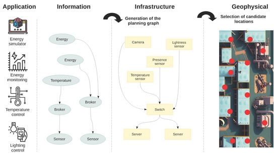
The proposed modeling is centered around the SmartParcels tool [23,24], a framework designed to develop plans for equipping specific areas within smart communities. The problem is divided into four layers—application, information, infrastructure, and geophysics—as shown in Figure 1.

The scenario unfolds as an optimization challenge, poised to maximize the overall utility of applications following the strategic deployment of IoT devices, edge servers, and network switches. Service utility is quantified through two essential dimensions: (i) coverage, which delineates the geographical scope where application events can be detected, and (ii) accuracy, which gauges the likelihood of accurately identifying those events.

Crafting an effective deployment strategy demands adherence to a series of stringent constraints. These include financial limitations for installation and operation as well as considerations of detection ranges, computing capacity, network bandwidth, and quality-of-service (QoS) expectations. Tackling the intricacies of application planning is seen as a challenging task, given the intricate interdependencies among four vital layers: the application layer, tasked with executing services; the information layer, responsible for managing data processing and transmission; the infrastructure layer, which encompasses vital hardware resources; and the geophysical factors, which significantly impact deployment feasibility and efficiency.

In this complex landscape, the quest for an optimal solution promises enhanced performance and a transformative leap in harnessing technology for better outcomes.

The solution to be developed will serve as a differentiator compared to other energy efficiency promotion solutions. It aims to optimize the quantity of equipment and components needed while considering factors such as functionality and coverage.

The formulated model focuses on a manufacturing facility comprising multiple distinct rooms, denoted as
$S$ , where each individual room is represented by
$s_{i} \in S$ . Within this industrial environment, a diverse set of applications
$A_{i}$ is required to support various operational tasks, with each specific application being identified as
$a_{i, j} \in A_{i}$ .

The industrial environment is formally defined as a tuple
$(S, A_{i} | \forall s_{i} \in S)$ , where
$S$ represents the set of rooms, and
$A_{i}$ denotes the set of applications associated with each room
$s_{i}$ . For modeling convenience, each room is represented by the coordinates of its geometric center.

The facility consists of a set
$L$ of candidate deployment points, which include conventional infrastructure elements, such as lighting systems, air conditioning units, and computing devices, alongside IoT components like environmental sensors, edge computing nodes, and network communication equipment. These elements serve as potential locations for application execution and data collection.

Since different applications contribute variably to operational efficiency, each room
$s_{i}$ is assigned a weight
$β_{i, j}$ for each required application
$a_{i, j}$ , indicating its relative priority within that space. It is assumed—without loss of generality—that the sum of weights across all applications in a given room satisfies
$\sum_{\forall a_{i, j} \in A i} β i, j = 1$ ,
$\forall s_{i} \in S$ . This weighting mechanism facilitates an optimized resource allocation strategy by reflecting the specific functional demands of each industrial zone.

Modeling must be conducted for an industry by considering all its rooms. Assuming the industry has 15 rooms, we can establish a model where
$| S | = 15$ and
$S = s_{1}, s_{2}, \dots, s_{15}$ . Let us further assume that one of these rooms, specifically room
$s_{1}$ , is an administrative room that requires two applications: temperature control and consumption monitoring. In this case, we can represent these applications as
$a_{11}$ and
$a_{12}$ . Furthermore,
$| A_{1} | = 2$ and
$A_{1} = a_{11}, a_{12}$ . This example is intended solely to illustrate the distribution of applications across rooms. The specific weight assigned to each application is detailed in the sections describing information and infrastructure flows, where factors such as coverage, accuracy, and resource allocation are considered. The model ensures that these weights reflect the relative importance of each application based on its functional role in the industrial environment.

The other elements of the model are described below.

3.1. Information Flows for an Application

Each application can be implemented using various combinations of sensor data from IoT devices and analytical algorithms on computing devices, such as edge servers. These devices are connected through directed graphs known as information flows. Different information flows for the same application enable planners to balance quality of service (QoS) with both deployment and operational costs. This allows for the selection of the most appropriate information flow to meet industry requirements.

To implement application

a_{i, j}

, a set of information flows

F_{i, j}^{i n f o}

can be adopted, with

f_{i, j, k}^{i n f o} \in F_{i, j}^{i n f o}

being the k-th information flow. More precisely,

f_{i, j, k}^{i n f o} = (V^{i n f o}, E^{i n f o})

is a directed weighted graph where

v \in V^{i n f o}

denotes a unit of information, which may consist of raw data or components of the communication middleware, and

e (u, v) \in E^{i n f o}

represents the data flow between these information units. Both the vertices and edges have associated weights. The weight of a vertex

w (v)

indicates the computing resources consumed by that unit of information, while the weight of an edge

w (e (u, v))

reflects the bandwidth consumption. Additionally, each information flow specifies the number of sensors needed; for example, three microphones are required for sound source detection using triangulation. Figure 2 illustrates how these information flows can be implemented in each application.

3.2. Infrastructure Flows Implementing an Information Flow

Each information flow can be deployed across various combinations of sensors, edge servers, and network switches, which are referred to as infrastructure flows. Different combinations of infrastructure flows associated with multiple information flows can result in varying levels of resource, or device, sharing. This allows for strategic planning to make use of resource reuse, leading to greater efficiency.

Each information flow
$f_{i, j, k}^{i n f o}$ can be represented by a set of infrastructure flows
$F_{i, j, k}^{i f r}$ , where
$f_{i, j, k, m}^{i f r} \in F_{i, j, k}^{i f r}$ denotes the m-th infrastructure flow. Let
$f_{i, j, k, m}^{i f r} = (V^{i f r}, E^{i f r})$ be a directed weighted graph, where
$v \in V^{i f r}$ represents a device and
$e (u, v) \in E^{i f r}$ represents the data flow between two devices. For our purposes, we consider various types of devices, such as sensors (for example, power meters or cameras), computing devices (like edge servers), and network switches (including LTE cells or Ethernet switches). The weights assigned to a vertex
$w (v)$ and an edge
$w (e (u, v))$ reflect the computing resources and network bandwidth they provide, respectively.

A tuple
$(F_{i, j}^{i n f o}, \forall f_{i, j, k}^{i n f o} \in F_{i, j}^{i n f o})$ encapsulates all information flows and their corresponding infrastructure flows for each application
$a_{i, j}$ .

Given a
$f_{i, j, k}^{i n f o}$ and a
$f_{i, j, k, m}^{i f r}$ , each processing unit
$v \in V^{i n f o}$ is assigned to a device
$v^{'} \in V^{i f r}$ through a specific function
$R (v) = v^{'}$ . Additionally, for a given edge
$e (u, v) \in E^{i n f o}$ ,
$〈 R (u), R (v) 〉$ represents the shortest path in
$f_{i, j, k, m}^{i f r}$ that includes the involved devices, reflecting the actual data flow at the infrastructure layer. For the sake of clarity, it is assumed that
$〈 R (u), R (v) 〉$ contains at least one network switch unless devices
$R (u)$ and
$R (v)$ are identical. If processes u and v operate on the same device, their network bandwidth is significantly higher, leading to the assumption that
$w (e (R (u), R (v))) = \infty$ .

Figure 3 illustrates how infrastructure flows can facilitate each type of information flow.

3.3. Planning Graph

Application deployment planning can be carried out by analyzing the flow of information and infrastructure. There are two types of deployments: (i) initial deployment, where no existing IoT infrastructure is in place (such as in a greenfield industry), and (ii) retrofit deployment, where IoT devices, edge servers, and network switches are already integrated (as seen in a growing industry).

An auxiliary structure known as a planning graph is created based on the following concepts. This planning graph is defined as a two-layer graph
$G^{p} = (V^{p}, E^{p})$ : the first layer
$G_{1}^{p} = (V_{1}^{p}, E_{1}^{p})$ consists of a set of information flows, while the second layer
$G_{2}^{p} = (V_{2}^{p}, E_{2}^{p})$ comprises a set of infrastructure flows. In both layers, flows can share vertices and edges. Additionally, a set of assignment edges
$E^{r}$ is defined, where each edge
$e (v, R (v))$ represents the assignment of
$v \in V^{i n f o} \subset V_{1}^{p}$ to
$R (v) \in V^{i f r} \subset V_{2}^{p}$ for
$f_{i, j, k}^{i n f o}$ and
$f_{i, j, k, m}^{i f r}$ . This planning graph can be denoted as
$V^{p} = V_{1}^{p}, V_{2}^{p}$ and
$E^{p} = E_{1}^{p}, E_{2}^{p}, E^{r}$ .

3.4. Infrastructure Geophysical Mapping Function

To identify candidate locations, a geophysical mapping function
$f (v)$ maps a vertex
$v \in V_{2}^{p}$ from the infrastructure layer of a planning graph
$G^{p}$ to each candidate location
$l \in L$ .

A tuple

t_{v} = (r_{v}^{t r}, r_{v}^{s i n}, τ_{v})

represents each device

v \in V_{2}^{p}

. The device’s transmission range is denoted by

r_{v}^{t r}

, while

r_{v}^{s i n}

indicates its detection range.

τ_{v}

specifies the type of device, which can be either a sensor, a compute unit, or a network device. If

τ_{v} \neq

“network”, then

r_{v}^{t r}

represents the transmission range of its associated network device u, denoted as

r_{v}^{t r} = r_{u}^{t r}, e (v, u) \in E_{2}^{p}

. Furthermore, multiple devices can be assigned to the same candidate location. For clarity,

V_{i, j, k, m}^{s i n}

is used to refer to the sensors of

f_{i, j, k, m}^{i f r}

(that is,

\forall v \in V_{i, j, k, m}^{s i n}, τ_{v} =

“sensor”). Figure 4 illustrates the geophysical mapping for an infrastructure flow. To identify candidate locations, a geophysical mapping function

f (v)

will associate a vertex

v \in V_{2}^{p}

of the infrastructure layer of a planning graph

G^{p}

with a potential candidate location

l \in L

3.5. Utility of a Service in an Infrastructure Flow

The Euclidean distance between two candidate locations

l_{1}, l_{2} \in L

is defined as

d i s t (l_{1}, l_{2})

. By definition, the Euclidean distance between two two-dimensional points

(x_{1}, y_{1})

and

(x_{2}, y_{2})

is given by Equation (1):

$\sqrt{{(x_{2} - x_{1})}^{2} + {(y_{2} - y_{1})}^{2}}$

(1)

Infrastructure flow is considered connected if all its devices are linked after mapping, i.e.,

d i s t (f (u), f (v)) \leq m i n (r_{u}^{t r}, r_{v}^{t r}), \forall e = (u, v) \in f_{i, j, k, m}^{i f r}

; otherwise, the flow is deemed unconnected. If

f_{i, j, k, m}^{i f r}

is connected, the service utility in a room

s_{i}

is determined by Equation (2):

$U (f_{i, j, k, m}^{i f r}, s_{i}) = A (f_{i, j, k, m}^{i f r}) \times P (V_{i, j, k, m}^{s e n}, s_{i})$

(2)

where
$A (f_{i, j, k, m}^{i f r})$ represents accuracy, while
$P (V_{i, j, k, m}^{s i n}, s_{j})$ signifies the probability of detection.

If
$f_{i, j, k, m}^{i f r}$ is not connected, then
$U (f_{i, j, k, m}^{i f r}, s_{i})$ is defined as 0. Each
$f_{i, j, k, m}^{i f r}$ that pertains to the application
$a_{i, j}$ includes a precision model
$A (f_{i, j, k, m}^{i f r})$ that varies based on the method used. For instance, detection based on presence sensors is generally more accurate for identifying presence than detection based on images.

The detection probability models used here, similar to those in SmartParcels, are based on the concept of attenuated truncated mode [25]. This concept indicates that the coverage measure becomes very small when the distance between a spatial point and a sensor is too large. In such cases, the coverage measure can be disregarded, allowing for approximations by truncating the coverage measure at greater distance values. This approach ensures that signal coverage is realistically represented, preventing overestimating utility in areas with limited sensor effectiveness. However, it is important to note that the current implementation focuses on planning rather than real-time adjustments. Future developments could integrate dynamic recalibration mechanisms, adapting detection strategies based on environmental conditions and signal propagation variations in real-time applications.

Initially, for a sensor

v \in V_{i, j, k, m}^{s i n}

, the probability is attenuated (or decayed) with increasing distance in

s_{i}, d i s t (f (v), s_{i})

and truncated by its detection range

r_{v}^{s i n}

. Therefore, if

d i s t (f (v), s_{i}) \leq r_{v}^{s i n}, \forall v \in V_{i, j, k, m}^{s i n}

, the average truncated attenuated detection probability, denoted as Y, is expressed by Equation (3) as follows:

$\bar{p} = \frac{\sum_{\forall v \in V_{i, j, k, m}^{s e n}} e^{- α_{v} * d i s t (f (v), s_{i})}}{∣ V_{i, j, k, m}^{s e n} ∣}$

(3)

where
$α_{v}$ is a parameter that is related to v. If this relationship does not hold, then
$\bar{p} = 0$ .

The detection probability is limited by the sensors’ detection range, as defined in Equation (4):

$P (V_{i, j, k, m}^{s e n}, s_{i}) = \{\begin{matrix} \bar{p}, & if d i s t (f (v), s_{i}) \leq r_{v}^{s e n}, \forall v \in V_{i, j, k, m}^{s e n}; \\ 0, & otherwise . \end{matrix}$

(4)

The definitions provided complete the concept known as the utility of a service. It is important to note that the proposed algorithms are not dependent on the mathematical properties of this utility. As a result, there is complete freedom to apply various models. For instance, one can enhance the analysis by incorporating non-line-of-sight detection ranges [26]. These scenarios occur when detection is possible despite obstacles blocking the direct line of sight, relying on signal reflections, diffractions, or scattering to reach the receiver.

3.6. Costs

Each device
$v \in V_{2}^{p}$ in the infrastructure layer is subject to two types of costs:

(i): deployment cost
$δ_{d e p l o y} (v, l)$ due to deploying the device v at the candidate location
$l \in L$ , and
(ii): operational cost
$δ_{o p} (v)$ due to maintaining its operation.

The deployment cost charged once, while the operational cost is recurring. Furthermore, we define
$B_{d p}$ and
$B_{o p}$ as the budgets for deploying and operating the devices. The operational cost refers to the ongoing expenses required to keep the device functioning, such as energy consumption, maintenance, software updates, and other associated costs necessary for its continuous operation.

3.7. Problem Formulation

Given the industry’s operational characteristics, the interaction between information and infrastructure flows, and the constraints regarding resource availability, the energy efficiency planning problem seeks to optimize the overall quality of services while adhering to predefined cost budgets. The objective is to derive an optimal planning graph, denoted as
$G^{p^{*}}$ , and determine the corresponding geophysical mapping functions
$F^{*} = f^{*} (v) | \forall v \in V_{2}^{p^{*}}$ that best allocate resources across the industrial environment.

More precisely, the problem involves selecting an optimal set of locations for deploying IoT devices, network infrastructure, and edge computing resources to enhance the energy efficiency without compromising system performance. This requires balancing multiple constraints, including power consumption, latency, computational capacity, and spatial deployment feasibility. The energy efficiency planning problem is formally structured as follows:

$Maximize \sum_{\forall s_{i} \in S} \sum_{\forall f_{i, j, k, m}^{i f r^{*}} \in G_{2}^{p^{*}}} β_{i, j} U (f_{i, j, k, m}^{i f r^{*}}, s_{i}),$

(5)

$subject to : \sum_{\forall v \in V_{2}^{p^{*}}} δ_{d e p l o y} (v, f^{*} (v)) \leq B_{d p},$

(6)

$\sum_{\forall v \in V_{2}^{p^{*}}} δ_{o p} (v) \leq B_{o p},$

(7)

$\sum_{\forall e (u, v) \in E^{r^{*}}} w (u) \leq w (v), \forall v \in V_{2}^{p^{a s t}},$

(8)

$\sum_{\forall e (u, v) \in E_{2}^{p^{*}}} w (e (u, v)) \leq \sum_{\forall e (v, u^{'}) \in E_{2}^{p^{*}}} w (e (v, u^{'})), \forall v \in V_{2}^{p^{*}},$

(9)

$w (e (u, v)) \leq min_{\forall e^{'} \in 〈 R (u), R (v) 〉} w (e^{'}), \forall e (u, v) \in E_{1}^{p^{*}} .$

(10)

The objective function in Equation (5) is designed to determine the optimal planning graph

G^{p^{*}}

and the corresponding geophysical mapping functions

F^{*}

that maximize the total utility of the system. This optimization process efficiently balances resource allocation, service quality, and energy consumption.

Budget constraints are enforced through Equations (6) and (7), which, respectively, limit the implementation cost

(B_{d p})

and the operational cost

(B_{o p})

. These constraints ensure that the deployment and ongoing management of the industrial infrastructure remain within financial feasibility.

To maintain computational efficiency, Equation (8) restricts every device

v \in V_{2}^{p^{*}}

, ensuring that its available computational resources are sufficient to process all assigned information units u. This constraint means that each device’s weight

w (v)

must be at least equal to the cumulative weight of all associated processing tasks, preventing system overloads and performance degradation.

Furthermore, Equation (9) guarantees that each device’s output bandwidth capacity is at least as high as its input bandwidth demand. This condition ensures smooth data transmission across the network, reducing bottlenecks and enhancing system responsiveness.

For every data stream

e (u, v) \in E_{1}^{p^{*}}

, Equation (10) enforces that the minimum bandwidth along the allocated communication path

〈 R (u), R (v) 〉

meets or exceeds the required bandwidth threshold. This constraint is required to maintain reliable data flow across the industrial IoT network, support real-time applications, and minimize latency issues.

On top of these definitions, the energy efficiency planning problem can be classified as a

NP

-hard optimization problem, which inherently resists approximation within a factor of

1 - 1 / e

. This complexity can be established by demonstrating a polynomial-time reduction from the well-known max K-cover problem [27] to a constrained version of the energy efficiency planning problem.

To achieve this reduction, consider a simplified instance where resource constraints are entirely removed by disregarding Equations (8)–(10). In this special case, each application is assumed to be associated with a single infrastructure flow, while deployment and operational costs are set to a uniform value of one. Additionally, both budget limits are defined as exactly K. Under these conditions, solving the energy efficiency planning problem is equivalent to selecting K infrastructure flows for a set of rooms in a way that maximizes overall service utility.

Since the max K-cover problem is

NP

-hard and has a polynomial reduction to this special case, the original energy efficiency planning problem retains the same computational complexity. Furthermore, as demonstrated by Feige [28], the max K-cover problem cannot be approximated within a factor better than

1 - 1 / e

unless

P = NP

. Consequently, this inapproximability threshold extends to the energy efficiency planning problem, reinforcing the inherent computational challenge associated with optimizing the energy efficiency under deployment and operational constraints.

4. Heuristic Solution

The smart space planning problem is decomposed into two subproblems targeting reducing complexity and avoiding redundant calculations: (i) geophysical mapping selection, which chooses promising mappings among infrastructure flows and candidate locations, and (ii) generation of planning graphs, which calculates mappings between information flows and infrastructure flows that maximize the overall service utility.

Let
$G^{p^{*}} = (V^{p^{*}}, E^{p^{*}})$ denote the optimized planning graph, where
$G_{1}^{p^{*}} = (V_{1}^{p^{*}}, E_{1}^{p^{*}})$ represents the set of information flows and
$G_{2}^{p^{*}} = (V_{2}^{p^{*}}, E_{2}^{p^{*}})$ defines the infrastructure flows. This decomposition is essential because identifying the optimal planning graph requires the continuous generation and assessment of geophysical mappings associated with
$G^{p^{*}}$ . Since these mappings remain largely static, a more efficient strategy involves storing and reusing them rather than recalculating them at each step.

Figure 5 illustrates the interdependence between these subproblems and the computational methods used to solve them. The Selection (SEL) algorithm prioritizes geophysical mappings that maximize service utility and communication reach, aiming to reduce the number of deployed devices. Meanwhile, the Maximum Reusability (MR) algorithm iteratively chooses infrastructure flows that optimize device utilization, minimizing redundancy and enhancing resource efficiency. Integrating these approaches, the proposed model balances service performance, network efficiency, and cost-effectiveness in energy-efficient planning.

Based on the results from [24], it was possible to develop a solution approach based on dynamic programming that generates the planning graph with maximum service utility. However, the execution time increases dramatically when the number of rooms, required applications, implementation methods (information flows and infrastructure), or candidate locations increases. Therefore, the optimal solution is unfeasible due to its extremely long time to complete. As a result, the algorithms presented represent a heuristic solution for each subproblem.

The first heuristic, SEL, is based on selection policies to eliminate less promising mappings. The policies contain the following intuitions: (i) MIFs with more significant utilities should be included earlier and (ii) MIFs with more excellent communication coverage should be included earlier.

For each

f_{i, j, k, m}^{i f r}

, the utility can be estimated by Equation (2) after mapping all equipment (assuming that the graph is connected). Similarly, the communication coverage of a network device can be estimated after mapping. Algorithm 1 presents the adopted heuristic, using M and N to represent the user-specified pruning criteria for utility and communication coverage, respectively.

Algorithm 1: SEL

(S, A, F^{i n f o}, F^{i f r})

input:: set of rooms (
$S$ ), applications (
$A$ ), information flows (
$F^{i n f o}$ ), and infrastructure flows (
$F^{i f r}$ ).
output:: promising set of geophysical mappings for possible infrastructure flows.

In the MR heuristic, instead of examining all possible combinations of MIFs, it iteratively (i) selects an application
$a_{i, j} \in \hat{A}$ to implement and (ii) merges an END
$\hat{F} \in M_{i, j, k, m}^{i f r}$ in the planning graph
$\hat{G} (K)$ according to the reusability of
$\hat{F}$ , where
$M_{i, j, k, m}^{i f r} \in {\hat{M}}_{i, j}$ . A reusability index was defined, considering the investment efficiency and the gain in communication coverage when merging
$\hat{F}$ .

Investment efficiency is the ratio between the application’s utility gain and the cost gain after merging

\hat{F}

into

\hat{G} (K)

. In other words, the more infrastructures are reused, the lower the costs will be with merging

\hat{F}

. Specifically, whether we choose

Δ U (\hat{F}, \hat{G} (K))

, and considering the application’s utility gain after merging

\hat{F}

into

\hat{G} (K)

, the cost gain is given by

$Δ δ (\hat{F}, \hat{G} (K)) = {\hat{δ}}_{d p} (K) - {\hat{δ}}_{d p} (K - 1) + {\hat{δ}}_{o p} (K) - {\hat{δ}}_{o p} (K - 1)$

(11)

Therefore, we have

$I_{e f f} (\hat{F}, \hat{G} (K)) = \frac{Δ U (\hat{F}, \hat{G} (K))}{Δ δ (\hat{F}, \hat{G} (K))}$

(12)

which is the investment efficiency of merging
$\hat{F}$ into
$\hat{G} (K)$ .

The current investment efficiency formula balances utility gain and costs in a structured industrial environment. However, we acknowledge that a more adaptive approach could be beneficial in environments with a highly variable application utility and resource costs. One potential adaptation would be introducing weight adjustments based on real-time demand fluctuations, prioritizing applications with a higher dynamic impact. Additionally, integrating cost prediction models could refine investment decisions by anticipating resource variations. Although this extension is not currently implemented, it represents a promising direction for future work, particularly for applications in heterogeneous or rapidly changing industrial contexts.

Communication coverage gain is determined by the locations of network devices. If a network device has greater communication coverage after deployment, fewer devices will be needed. Let

L_{c o v} (K) \subset L

be the candidate locations in the communication coverage of network devices in

\hat{G} (K)

. The communication coverage gain after merging

\hat{F}

into

\hat{G} (K)

is given by

$I_{c o v} (\hat{F}, \hat{G} (K)) = L_{c o v} (K) - L_{c o v} (K - 1)$

(13)

The reusability index is defined as a weighted sum of the investment efficiency and communication coverage gain when merging an FIM

\hat{F}

into the intermediate planning graph

\hat{G} (K)

. Let

α_{e f f}

and

α_{c o v}

be the weights of the investment efficiency and communication coverage gain, respectively. The reusability index is written as

$I (\hat{F}, \hat{G} (K)) = α_{e f f} I_{e f f} (\hat{F}, \hat{G} (K)) + α_{c o v} I_{c o v} (\hat{F}, \hat{G} (K))$

(14)

Without the loss of generality, it is assumed that
$α_{e f f} + α_{c o v} = 1$ .

With these definitions, MR starts with an empty planning graph

\hat{G} (0)

and iteratively selects an application

a_{i_{j}} \in \hat{A}

to implement by merging an END

\hat{F} \in M_{i, j, k, m}^{i f r}

in the current intermediate planning graph

\hat{G} (K)

(as established in Algorithm 2), where

M_{i, j, k, m}^{i f r} \in {\hat{M}}_{i, j}

Algorithm 2: MR

(S, A, F^{i n f o}, F^{i f r})

input:: set of rooms ( $S$ ), applications ( $A$ ), information flows ( $F^{i n f o}$ ), and infrastructure flows (
$F^{i f r}$ ).
output:: planning graph.

Eng 06 00053 i002

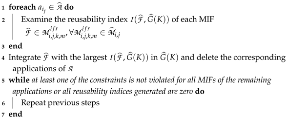
When viewing Lines 1 to 3 (Algorithm 2), for each application
$a_{i_{j}} \in \hat{A}$ , it can be seen that the algorithm examines the reusability index
$I (\hat{F}, \hat{G} (K))$ for each END
$\hat{F}$ within the set of possible mappings
$M {i, j, k, m}^{i f r}$ , where
$\hat{M} i, j$ represents the set of all mappings for the considered application. In Line 4 (Algorithm 2), the END
$\hat{F}$ with the highest reusability index
$I (\hat{F}, \hat{G} (K))$ is then incorporated into the planning graph
$\hat{G} (K)$ . Applications corresponding to this END are excluded from the set
$A$ , indicating that their infrastructure needs have already been met.

The process repeats the evaluation and selection steps as long as at least one of the constraints is not violated for the MIFs of the remaining applications, or until all calculated reusability indices are zero. This strategy ensures that planning continues to optimize component reuse without violating operational or design constraints. As output, the algorithm produces a planning graph representing the infrastructure and application mapping, prioritizing component reuse.

To establish the convergence of our heuristic methodology, we validate two fundamental characteristics: (i) each successive step enhances the function
$U (G^{p^{*}})$ , and (ii) these enhancements gradually diminish, yielding convergence.

Initially, observe that the functional expression in the optimization challenge is expressed as

$U (G^{p^{*}}) = \sum_{\forall s_{i} \in S} \sum_{\forall f_{i, j, k, m}^{i f r^{*}} \in G_{2}^{p^{*}}} β_{i, j} U (f_{i, j, k, m}^{i f r^{*}}, s_{i})$

where
$U (f_{i, j, k, m}^{i f r^{*}}, s_{i})$ represents the utility of a selected infrastructure flow at room
$s_{i}$ , and
$β_{i, j}$ is a weighting factor for each application. The MR heuristic iteratively selects a FIM
$\hat{F}$ that maximizes the reusability index. Since the heuristic always selects
$\hat{F}$ such that it improves utility, it follows that

$U (G^{p^{*} (t + 1)}) \geq U (G^{p^{*} (t)}), \forall t .$

This characteristic guarantees that the efficacy function exhibits monotonic growth across iterations.

Next, we demonstrate that these improvements attenuate, culminating in convergence. Let

Δ U_{t}

represent the utility gain at iteration t, defined as

$Δ U_{t} = U (G^{p^{*} (t + 1)}) - U (G^{p^{*} (t)}) .$

Initially, when many high-impact infrastructure flows are available,

Δ U_{t}

is relatively large. However, as the number of remaining candidate FIMs decreases, additional selections yield redundancies due to overlapping mappings, reducing their incremental contribution to the utility. This behavior can be modeled as an exponential decay in utility gain as follows:

$Δ U_{t} = c \cdot Δ U_{t - 1}, where 0 < c < 1 .$

Since

Δ U_{t}

approaches zero as

t \to \infty

, we conclude that

$lim_{t \to \infty} Δ U_{t} = 0 .$

Finally, because

U (G^{p^{*}})

is both monotonically increasing and bounded above by the maximum achievable utility under budgetary and infrastructural constraints, the Monotone Convergence Theorem [29] guarantees that

U (G^{p^{*}})

converges to a finite value as follows:

$lim_{t \to \infty} U (G^{p^{*} (t)}) = U^{*} .$

Thus, we have established that the heuristic progressively achieves an optimal or near-optimal configuration, ensuring convergence while maximizing energy efficiency throughout industrial environments.

Implementation

The proposed solution was implemented as a prototype that was made available through a Web API. The objective was to develop a flexible application for both local and cloud infrastructure. Based on this, the implemented architecture is presented in Figure 6.

The first component is the user interface, which is designed to enable modeling and planning. This interaction occurs through the REST API. User models were validated according to the specifications intended for IoT models. This process is based on standards and specifications developed to facilitate interoperability and simplified data exchange between devices and systems in IoT environments.

Among the standards used, a large part is from [30], which is a collaborative initiative that aims to improve data models aimed at IoT. The data models are compatible with FIWARE version 2 [31] and Next-Generation Service Interface-Linked Data (NGSI-LD) [32] specifications, enabling their use by these standards. They encompass detailed definitions of properties, attributes, and relationships between various data entities, ensuring that information is not only accessible but also meaningful and readily usable across diverse systems. In total, 15 application domains were available, and models from 4 of them were used: Smart Energy, Smart Cities, Smart Robotics, and Smart Sensing.

In addition to Smart Data Models, schemas from [33] are used, which is a collaborative initiative led by large search engines aiming to structure information on the Internet through a standardized set of tags via Extensible Markup Language (XML).

To represent information and infrastructure flows, ref. [34] was used, which is a convention used to describe the data structure in graphs using the JSON format, facilitating data storage, manipulation, and transfer. Figure 7 summarizes the models used for data representation.

After validating the models, planning is performed using the heuristic solution described in the previous section.

The industry and its rooms are represented using GeoJSON [35], an open standard format designed to represent simple geographic features, along with their non-spatial attributes using JSON. Each candidate location is represented by the geographic coordinates of its location and deployment cost for each type of equipment in that location.

In information and infrastructure flows, each node is assigned a role that specifies its role. Vertices can be classified as sensor, representing sensors or any data collection device, network for component parts of the network, or compute, indicating devices with processing capacity. For vertices categorized as sensors, attributes list the data types that a device can collect.

The attributes that were introduced were r_tr and r_sen, which represent the transmission range ( $r_{v}^{t r}$ ) and sensing range ( $r_{v}^{s i n}$ ), respectively. In addition, precision_model was introduced as a representation of the precision model
$A (f_{i, j, k, m}^{i f r})$ . The procedure starts by selecting all possible geophysical mapping functions for each room, considering the sensors whose sensing area includes part of the room. In this analysis, candidate locations in the room and external locations are considered, as long as the room is in the sensing coverage area of a sensor in these locations.

The application was implemented in Python using the Django framework [36]. The choice for these tools was made because Python has a clear and readable syntax and is a robust option with a vast number of libraries available.

In the implementation, Shapely and Geopy libraries were used in Python 3.9. Shapely is used to manipulate and analyze plane geometry. It allows for the creation, manipulation, and analysis of geometries in addition to performing operations such as union, intersection, and difference on geometric objects. On the other hand, Geopy provides a simple and consistent interface for performing various geographic operations, such as geocoding, distance calculation between geographic points, and route calculation between locations. Moreover, it is often used in applications involving geographic data analysis, geolocation, and geocoding.

5. Performance Evaluation

The performance evaluation of our proposed smart space planning framework focuses on assessing the system scalability and cost-effectiveness in industrial environments. Using the simulated scenarios, we evaluated the efficiency of our IoT-based planning model. We employed a multifaceted evaluation that included scalability and cost-effectiveness analysis. By implementing optimized information and infrastructure flows, the system demonstrated consistent efficiency gains even as the number of deployed devices increased.

5.1. Setup

The experiments were implemented using a data generator to simulate data on industries and applications. The goal was to create a structured representation of the industry’s physical space and operational processes to simulate possible scenarios for using the proposed solution.

The total area of the specified physical space is divided into functional categories, such as production, offices, utility and storage, ensuring that the spaces are proportional to an industry’s typical needs. Each generated room has attributes, such as size, occupancy capacity, type of functional area, and geographic location.

Specific applications were also created for each room by considering the following possibilities: (A) detection of mechanical failures, abnormal vibrations, or compressed air leaks in industrial equipment through acoustic sensing; (B) monitoring of emissions in boilers and thermal processes through smoke sensing; (C) monitoring of the efficiency of ventilation systems through air quality sensing; (D) detection of overheating in machines or industrial processes through temperature sensing; and (E) lighting and cooling control through presence detection.

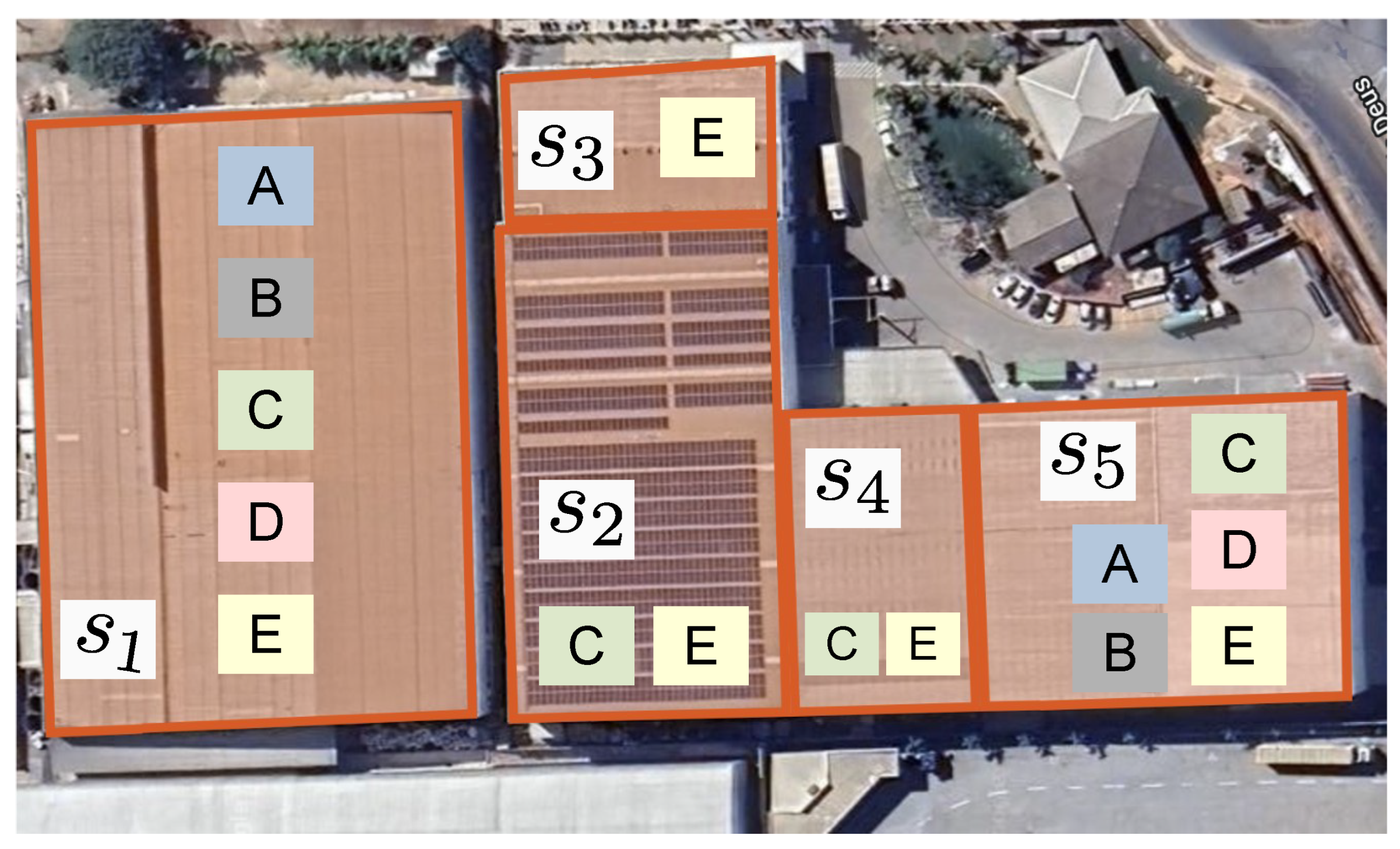
The experiment was modeled on a typical industrial setup, featuring functional spaces commonly found in industries worldwide. The physical plant was divided into five distinct rooms ( $s_{1}$ to
$s_{5}$ ). The Brazilian case was utilized solely to demonstrate the applicability of the solution. This division aims to simulate the industrial environment in detail, reflecting the typical requirements for evaluating the proposed IoT solution. The rooms were categorized as follows:

•: $s_{1}$ : Production Area: represents the majority of the space, housing essential industry production processes.
•: $s_{2}$ : Storage Area: designated for storing materials and finished products.
•: $s_{3}$ : Utilities’ Area: this area is intended for operational support, such as production support machines and general utilities.
•: $s_{4}$ : Office: place dedicated to administrative and management activities.
•: $s_{5}$ : Other Production Area: this area complements the production processes and may include specific production lines.

Specific IoT applications were simulated for each of these areas to meet the functional and operational demands of each space:

•: $s_{1}$ and
$s_{5}$ (Production): Applications A (detection of mechanical failures, abnormal vibrations, or compressed air leaks), B (monitoring of emissions in boilers and thermal processes), C (monitoring of the efficiency of ventilation systems), D (detection of overheating), and E (lighting and cooling control).
•: $s_{2}$ (Storage): Applications C (monitoring of ventilation efficiency) and E (lighting and cooling control).
•: $s_{3}$ (Utilities): Application E (lighting and cooling control).
•: $s_{4}$ (Office): Applications C (monitoring of air quality) and E (lighting and cooling control).

The floor plan presented in Figure 8 illustrates the layout of these rooms and their respective applications, simulating real scenarios and allowing for a practical evaluation of the IoT deployment planning tool.

Wi-Fi and Lora were considered for network communication. The equipment parameters used to deploy the applications were the same as those adopted in [24], as listed in Table 1. However, in our representation, we include the memory requirement by considering a buffer of 10 s. Moreover, hertz (Hz) measures the computing requirements by converting bits per second (bps) using
where

•: $f_{Hz}$ is the frequency in hertz (Hz);
•: $R_{bps}$ is the transmission rate in bits per second (bps);
•: N is the number of bits transmitted per cycle (we assume it as 64).

Figure 8.
Application deployment plan considered in the experiment.

Table 1.
Parameters used in the experiments [24].

Parameters		Values
Bandwidth consumption	Image	10 Mbps
	Motion sample	1.92 Kbps
	Emission reading	0.64 Kbps
	Sound	128 Kbps
Computing resource requirement	Image	1.25 MHz
	Motion sample	60 Hz
	Emission reading	20 Hz
	Sound	6 KHz
Memory requirement	Image	1.25 GB
	Motion sample	240 B
	Emission reading	80 B
	Sound	16 KB
Computing resource	Edge server	6.8 GHz (4 × 1.7 GHz)
Transmission range and bandwidth	WiFi AP	50 m/100 Mbps
Transmission range and bandwidth	Lora gateway	1 km/50 Kbps
Sensing range	Camera	15 m
	Motion sensor	10 m
	Gas sensor	600 m
	Microphone	300 m
Sensing parameter $α_{v}$ in Equation (3)	All sensors	Reciprocal of sensing range

Regarding information flow, two patterns were considered, as illustrated in Figure 9: a single source of sensing data that sends information to an analytical model or multiple sources of sensing data.

Infrastructure flows are generated from each information flow, as specified in the patterns in Figure 10, and a sensor is established for each source of sensing data and an edge server for each analysis model. In addition, one or more network devices were considered.

The values established in [24] were also maintained for the cost of implementing and operating equipment. However, corrections were applied due to inflation, based on what was established by the U.S. Bureau of Labor Statistics [37]. The adjusted values are presented in Table 2.

The number of candidate locations was established using the Brazilian standard ABNT NBR 5410 [38], which defines standards for electrical installations. According to this standard, one power outlet point is sufficient if the area reaches 6 m². One outlet point is required for every 5 m, or a fraction thereof, of the perimeter if the area of the room or dependency is greater than 6 m²; these points should be spaced as evenly as possible.

The proposed solution was developed to be geographically neutral, relying on universal energy efficiency principles and IoT deployment. This neutrality ensures that the solution can seamlessly adapt to industries with varying infrastructural, economic, and regulatory conditions. Therefore, this Brazilian case study served as an illustrative example, and the model can be readily applied to other regions, supported by its modular and flexible architecture.

The experiments were conducted by varying the following parameters: (i) number of applications per room, (ii) number of information flows per application, (iii) number of infrastructure flows per information flow, (iv) deployment and operation budgets, and (v) MR weights to study their implications on various performance metrics.

5.2. Experimental Results

Figure 11 presents the results of running the tool for the considered scenario. When analyzing the implementation cost of the number of flows (Figure 11a), both information and infrastructure, it is possible to observe trends that reveal the interdependence between these parameters. The data suggest that, as the number of flows increases, the cost also tends to increase proportionally. This behavior is expected because more information flows imply an increase in the number of detection and communication devices required to ensure application coverage and reliability.

Similar behavior was observed when analyzing the service utility of the number of flows (Figure 11b). As the number of flows increases, the utility tends to grow. This behavior is justified by the greater density of information collected and transmitted, which expands the application’s ability to detect events in a broader area with greater precision. However, utility tends to show decreasing marginal gains as the flows reach a certain level. In other words, after a certain point, the addition of new flows does not generate a significant increase in utility, indicating the presence of redundancies.

Regarding coverage, it is possible to observe a direct and significant relationship in Figure 11c, which reveals how the increase in flows affects the IoT solution’s ability to monitor geographic areas and expand event detection. The coverage tends to grow proportionally when the number of flows increases, especially in the initial stages. This behavior occurs because additional flows allow the inclusion of more devices and sensors, increasing network density and expanding the geographic reach of the application. However, as the flow continued to grow, the rate of gain in coverage decreased. This behavior is explained by the fact that after reaching a specific density of sensors, additional flows begin to overlap areas that are already covered, resulting in redundancy and not a significant gain in coverage.

On the other hand, investment efficiency shows a decreasing trend as the number of flows increases (Figure 11d). This behavior reflects a relationship of diminishing returns in which the growth of the utility obtained does not keep pace with the proportional increase in costs. In other words, adding new flows contributes to significant gains; however, these gains become progressively smaller as flows increase, whereas costs continue to grow linearly or exponentially.

When analyzing the relationship between the covered locations (Figure 11e), a particular behavior is observed when

α_{e f f}

= 1 and

α_{c o v}

= 0. In this configuration, the covered location metric does not reach a value of 5, whereas all other weight configurations manage to reach or exceed this value. This result indicates that the system’s ability to expand the served geographic area by exclusively prioritizing efficiency over coverage, which is limited even with increased flows. Furthermore, as the number of flows increased in this specific configuration, the number of covered locations increased at a steadier pace than in the other weight configurations. This behavior suggests that, even under the exclusive prioritization of efficiency, the flow increase still contributes to expanding coverage but is less effective. The absence of weight attributed to coverage limits the impact of new flows on the expansion of the served geographic area. In contrast, in configurations where

α_{c o v}

has positive values, the system can simultaneously optimize efficiency and coverage, achieving higher values for covered locations. This result occurs because the weight attributed to coverage directs resources to expand the system’s performance geographically, maximizing utility and the area served.

The experimental results indicate that the proposed model demonstrates scalability to a certain extent, particularly regarding the increasing number of deployed devices and their impact on cost, utility, and coverage. The heuristic-based approach optimizes resource allocation, ensuring efficient device reuse while minimizing redundancy. However, we acknowledge that the scalability assessment did not cover all potential factors, such as extreme increases in the number of rooms or highly heterogeneous industrial environments. Nevertheless, given that the solution is designed for planning within a specific industrial context, we do not anticipate scenarios requiring an exceptionally high number of rooms. The model primarily focuses on optimizing the energy efficiency within predefined industrial spaces rather than handling large-scale deployments across multiple facilities. Future work could explore adaptations to enhance scalability for broader applications beyond the targeted industrial setting.

6. Final Remarks

One of the primary motivations for the solution presented in this work was the increasing complexity of challenges related to energy production, distribution, and consumption. The solution seeks to contribute to the energy efficiency in smart spaces in the context of Industry 4.0. The global demand for solutions that combine sustainability and technological innovation requires models capable of integrating advanced technologies, such as the IoT, artificial intelligence, and cloud computing, to promote more efficient, connected, and resilient industrial operations.

In this scenario, this study presented an adaptation of the SmartParcels framework, which constitutes an integrated model for planning smart spaces, combining sensing, communication, computing, and application layers. The model allows for the optimization of resource utilization and for maximizing the utility of services, respecting cost constraints and ensuring high energy efficiency. Specific heuristics were used to select promising geophysical mappings and maximize the reuse of devices, promoting economic and environmental sustainability. The experimental results demonstrated that the proposed solution is scalable and viable for large-scale applications across diverse industrial contexts. By not assuming region-specific characteristics, the model ensures adaptability to different industries and geographical regions.

Our analysis reveals that implementing a structured methodology for selecting information and infrastructure flows as well as heuristic-based optimization techniques yields substantial efficiency improvements. These insights provide valuable practical guidance for manufacturing, logistics, and industrial automation sectors navigating the transition to Industry 4.0 paradigms. Using our approach, the strategic allocation of IoT devices demonstrates multiple tangible benefits: (i) reduced energy consumption across industrial systems, (ii) minimized infrastructure expenditure, and (iii) enhanced system scalability for future expansion.

The results suggest that organizations can apply these methodologies to achieve optimal resource utilization while maintaining operational effectiveness. This balance between efficiency and performance represents a critical consideration for industries seeking competitive advantages in increasingly digitized operational landscapes.

However, some challenges pave the way for future work. It is important to note that the proposed solution focuses exclusively on the planning phase of smart spaces, specifically the design and deployment of IoT infrastructure to optimize energy efficiency. It does not address tasks or costs associated with the real-time execution of applications within these spaces, which remains outside the scope of this work.

Additionally, the model does not differentiate between constant and variable energy consumption scenarios. For example, energy usage in production areas may vary depending on production volume, while offices and utilities typically exhibit more constant consumption patterns. Future research should incorporate these dynamic factors to improve the model’s applicability to real-world industrial contexts. Furthermore, the model could be adapted to various sectors, such as precision agriculture, healthcare, and transportation, expanding its applicability and relevance. Another possibility would be to incorporate algorithms based on machine learning or artificial intelligence to improve the accuracy and adaptability of planning decisions, especially in dynamic scenarios with high device heterogeneity.

Additionally, validating the model in real industrial environments is essential to confirm its robustness and ability to meet complex demands. Such validation would enable a deeper analysis, including statistical hypothesis testing and sensitivity analyses, which are not feasible within the current simulation-based framework. This analysis could involve case studies in diverse industries, providing insights into operational efficiency, sustainability gains, and return on investment while addressing dynamic energy consumption patterns.

Finally, creating more intuitive interfaces and visualization tools could facilitate the model’s adoption by multidisciplinary teams, promoting its integration into strategic decision-making processes. Thus, this work lays the foundations for developing even more advanced solutions aligned with contemporary demands for innovative, sustainable, and efficient industrial operations.

Source link

Viviane Bessa Ferreira www.mdpi.com

Greenberg News

Planning Energy-Efficient Smart Industrial Spaces for Industry 4.0

1. Introduction

2. Related Work

3. Proposed Modeling

3.1. Information Flows for an Application

3.2. Infrastructure Flows Implementing an Information Flow

3.3. Planning Graph

3.4. Infrastructure Geophysical Mapping Function

3.5. Utility of a Service in an Infrastructure Flow

3.6. Costs

3.7. Problem Formulation

4. Heuristic Solution

Implementation

5. Performance Evaluation

5.1. Setup

5.2. Experimental Results

6. Final Remarks

Greenberg

1. Introduction

2. Related Work

3. Proposed Modeling

3.1. Information Flows for an Application

3.2. Infrastructure Flows Implementing an Information Flow

3.3. Planning Graph

3.4. Infrastructure Geophysical Mapping Function

3.5. Utility of a Service in an Infrastructure Flow

3.6. Costs

3.7. Problem Formulation

4. Heuristic Solution

Implementation

5. Performance Evaluation

5.1. Setup

5.2. Experimental Results

6. Final Remarks

Related Posts

A Comparative Approach in an Emerging European Context

Pathophysiological Mechanisms and Clinical Therapy

Chumash Heritage National Marine Sanctuary

Greenberg