Remote-Sensed Spatio-Temporal Study of the Tropical Cyclone Freddy Exceptional Case

1. Introduction

Tropical cyclones involve high intensification of low-pressure systems, generally characterized by strong winds, heavy rainfall, and thunderstorms, in a synoptic rotational motion. A key role in the evolution is associated with the core of the storm with a warm air column (eye), which is surrounded by a shell-like zone where the most destructive winds and precipitation occur (eyewall) [1]. The Saffir–Simpson scale is widely used to categorize these events, with their intensification and weakening described based on variations in the vertical wind shear, short-time maximum sustained wind, and pressure minimum parameters [2,3,4].

Starting in a favorable thermodynamical environment, sustained convection leads to the formation of a surface vortex, which then intensifies until the peak of intensity, drawing significant energy from the ocean, which later may weaken due to unfavorable conditions like cold sea-surface temperatures, strong vertical wind shear, or landfall [5,6]. Multi-scale interactions influence the TC’s development, movement, structure, and intensity changes [7]. In the North Indian Ocean basin, which includes the Bay of Bengal and the Arabian Sea, these cyclones primarily form between April and December. Some climatological studies confirm that in this area the impact of rising sea-surface temperatures (SSTs) and the vertical profiles of the heat potential, particularly in the Arabian Sea, play a key role in the formation of very intense tropical cyclones [8,9] and they are inferred using satellite remote sensing applications.

Recent advances in the capability of new satellite sensors show several applications for observing tropical cyclone structure, wind fields, and temporal evolution [10]. This study is based on the exploitation of a large database collected from geostationary (GEO) sensors that provides high spatial, temporal (from 1 min to 10 min), and spectral resolution. Data and imagery are collected from ESA/EUMETSAT GEO missions of Meteosat Second Generation-8 (IODC) (MSG-8) by exploiting the products of the SEVIRI radiometer in thermal infrared (TIR) spectral channels [11,12]. TIR spectral data have been effectively used in detecting extreme atmospheric and geological events, such as volcanic eruptions, ash cloud tracking, and extreme rainfall [13,14,15]. In this study, SEVIRI’s TIR products are utilized to analyze the spatio-temporal evolution of Freddy tropical cyclone—one of the most powerful and long-lived tropical cyclones recorded during the 2023 Indian Ocean cyclone season [16,17,18]. With its 36 days of life, Freddy is catalogued as the longest-lasting tropical cyclone ever recorded worldwide, making it the producer of the most accumulated cyclonic energy of any other individual tropical cyclone globally. It breaks the record of precipitation spreading from the south of Indonesian archipelago until the Mozambique channel and then all over the ocean [19].

The total GEO database used for this investigation allowed an analysis of 12 days of Freddy’s evolution represented in 1152 TIR images. With these products, a spatio-temporal analysis of the dynamical evolution of the tropical cyclone was carried out using the Proper Orthogonal Decomposition (POD) technique, extending the methodology applied for the Faraji hurricane investigation in [20,21]. For a turbulent fluid which is neither homogeneous nor isotropic, the Fourier analysis in normal modes does not produce optimal results. In particular, the most energetic structures of the flow are not “plane waves” in the Fourier sense, but they assume the form of localized structures called coherent structures. They emerge dynamically in flow evolution, persisting and interacting with their surroundings. For example, in wall-bounded turbulent flows, such structures are continuously created and destroyed near the wall region, undergoing a cycle of creation, evolution, and destruction (ejection-sweep-burst), leading to effective energy dissipation and significantly influencing the overall flow dynamics. By referring to tropical cyclones as nonhomogeneous and nonisotropic scenarios, POD represents a valuable tool for obtaining more consistent information on the spatio-temporal dynamics of such structures, especially considering their different aspects and stages. It is a procedure for extracting empirical bases to construct a modal decomposition from an ensemble of signals, and it has been introduced in the context of turbulence for investigating dynamical systems without nonlinear or numerical limitation [22]. It has the capability to decompose the original field (scalar or vector), extracted from the data, into a basis of empirical eigenfunctions by diagonalizing the autocorrelation matrix in the whole domain. In particular, in a generic nonhomogeneous flow, POD can capture persistent structures in their life cycle, and for this reason, it is often preferred to the traditional expansions (such as Fourier or Wavelet) because it preserves the flow behavior at the boundaries of the spatial domain in order to describe a turbulent field with spatial and temporal structures in a rigorous mathematical background [23]. POD solutions represent, on average, the maximization of energy content in the empirical basis for spatial and temporal components, separately, of the dynamics of the system, thanks to their property of orthonormality [24,25,26]. With the POD expansion, it is then possible to reconstruct the original field at different scale ranges associated with the maximum energy content distribution from the big central structure of the field representing the tropical cyclone to the small scales structures of its evolution.

Looking at the diagnostics of the Freddy life cycle from February 10th to 21th, in the first third of its total period of evolution, the application of POD is performed on 2D scalar fields of cloud-top temperature

T_{e f f}

and atmospheric pressure field P at a fixed height

H = 500

m above sea level. Both parameters are computed from the brightness temperature

T_{b}

value contained in the SEVIRI images in the TIR spectral channels. The analysis proceeds in three different phases. In the first part, by exploiting the total SEVIRI database, POD is applied on the temperature and pressure fields, dynamically varying the spatial domain during all 12 days. More precisely, the grid

(l o n, l a t)

is moved over the analyzed period to follow the displacement of the cyclone. With the aim of maintaining the same dimensions of the grid, only varying the geographical coordinates for the position of the cyclone, a spatial reconstruction algorithm is performed on the tracking of Freddy’s central eye, interpolating its temporal evolution with the resolution of the satellite products. In particular, the eye coordinates are provided by the International Best Track Archive for Climate Stewardship (IBTrACS) database [27] and consist of 3 hourly timesteps, which are then integrated with the 15-min timesteps associated with the SEVIRI images. The second part is based on the application of POD to eight different 24-h intervals of the total period, focusing on the spatio-temporal energy distribution in the modes associated with the transition of the Freddy stages.

The analyses are performed on four weakening transitions (from higher to lower intensity categories) and on four strengthening transitions (from lower to higher categories) in order to highlight and compare the energy distributions in the spectra over the ocean crossing of Freddy. The last part is a focus on the 24 h of the maximum intensification stage of Freddy, the period in which the tropical cyclone reached the status of hurricane, and in the fifth category of the Saffir–Simpson intensity scale. This investigation provides the POD expansion of the

T_{e f f}

field during the 24 h of February 19th, when the Freddy upgrade to very intense tropical cyclone (fifth-category hurricane) was recorded by Météo-France with the Dvorak technique [28] before approaching the Mascarene Islands.

The results obtained from the decomposition in this phase were taken into account for a comparison with the results of Faraji, representing the last fifth-category Indian Ocean tropical cyclone before Freddy. With this comparison, the possibility to find the key points of the characteristic behavior of the spatio-temporal dynamics of Indian Ocean TCs can be highlighted from the POD energy spectra results in order to focus on the analogies of the role of the emerging structures in the different scale ranges of the maximum intensity of these events in this geographical area.

2. Methods

SEVIRI is a passive radiometer onboard the GEO MSG-8 IODC satellite platform whose orbit is positioned about 36,000 km above the Earth’s surface. Its flight is an operational ESA/EUMETSAT program that provides near-real-time images of weather processes over the Indian Ocean, by tracking clouds and water vapor features with a full-disk coverage [11]. It has low spatial resolution (pixel dimension of 3 km at nadir) but very high revisiting temporal cycles (5–60 min).

The High Rate SEVIRI satellite mission was chosen for the product acquisition, selecting the IR10.8 Thermal InfraRed (TIR) spectral channel. Consdering 12 days of evolution of the Freddy tropical cyclone, with a 15-min acquisition timestep of the products, we collected 1152 images. Each image, acquired in raw format, initially underwent a preprocessing phase, which consists of georeferencing [29]. This phase is based on the use of the Nearest Neighbor interpolation algorithm, consisting of the geometrical redistribution of the pixels, reprojected and resized on the ellipsoid system UTM WGS-84, without alteration of the data.

The new products have a spatial domain of

350 \times 350

pixels, with geographical coordinates varying according to Freddy’s displacement. Each pixel contains Digital Number (DN) data, which are converted into radiance

L_{λ}

using a linear relationship based on sensor calibration parameters.

T_{b}

is derived by inverting Planck’s law (Equation (1)) [30,31], assuming unitary emissivity to neglect reflected radiance along the line of sight and considering the dependence on the central wavelength of the TIR spectral channel.

$T_{b} = \frac{h c {(k λ)}^{- 1}}{ln (\frac{2 h c^{2} ϵ λ^{- 5}}{L_{λ}} + 1)} .$

(1)

Since $T_{b}$ represents sensor-measured radiation rather than a physical quantity, a postprocessing algorithm is applied to retrieve the cloud system’s altitude H and effective temperature $T_{e f f}$ . This is achieved through a system of linear equations that relate brightness temperature with dew point ( $T_{D} = T_{b}$ ) and altitude (Equation (2)) in the conditions of the air temperature drop of 9.84 °C per 1000 m of altitude and the dew point drop of 1.82 °C per 1000 m of altitude, respectively, and with $T_{a m b}$ as a time-dependent variable corresponding to the air temperature at 2 m above sea level from fifth-generation ECMWF atmospheric reanalysis (ERA5) data.

$\{\begin{matrix} H = (T_{b} - T_{a m b})) / (- 0.00802) \\ T_{e f f} = - 0.00984 [(T_{b} - T_{a m b})) / (- 0.00802)] + T_{a m b} \end{matrix}$

(2)

The atmospheric pressure P is subsequently estimated using an exponential law (Equation (3)), where the scale height $α$ is a characteristic vertical dimension of mass distribution, typically variable with temperature variations between 8 km (in the layers near the surface) and 6 km (highest and coldest regions of the atmosphere) [2,3], and $P_{0} =$ 1013.25 hPa is the surface pressure under standard conditions.
This methodology enables the direct retrieval of temperature and pressure fields from satellite data, providing insights into their spatial and temporal variations.

The technique chosen in this work for this type of analysis is Proper Orthogonal Decomposition (POD), which is widely used for several systems with significant dynamical properties [32,33,34,35,36], in which an optimal investigation comes out by decomposing a scalar or vector field defined on a specific space–time domain.

For the case of the Freddy tropical cyclone, the POD expansion was applied following the procedure of [20,21], on the cloud-top temperature

T_{e f f}

and atmospheric pressure P scalar fields. Meteorological history of Freddy shows the overpass all over the Indian Ocean during its 36 days of total life cycle, specifically in the period chosen for this analysis. 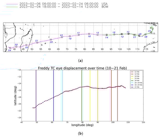The fields were reconstructed using a dynamical grid centered around the cyclone’s eye based on the database provided by IBTrACS, specifically from the United States (USA) and Australian Bureau Of Meteorology (BOM) agencies, with an interpolation of the 3 hourly resolution with a cubic spline method used to reproject the position of the eye of the cyclone to a resolution of 15 min. The POD expansion is defined as follows:

$F (x, y, t_{k}) = \sum_{j} a_{j} (t_{k}) ϕ_{j} (x, y)$

(4)

where f is the examined scalar field, $a_{j} (t)$ are time-dependent modal coefficients, and $ϕ_{j} (x, y)$ are basis functions which depend on space variables. Equation (4) allows for the factorization of the spatial and time dependencies of the field that leads to a separate evaluation of the spatial and temporal behavior. The POD eigenfunctions are obtained by solving a Fredholm integral equation, solved with the use of a numerical code [24,25,26], which yields the optimal basis functions and their corresponding eigenvalues $λ_{j}$ representing the energy content of each mode.

The eigenfunctions $ϕ_{j} (x, y)$ are obtained from time-averaged auto-correlation and consist of a mutually orthogonal form, and the eigenvalues $λ_{j}$ represent the average energy content of the POD modes. The partial sums of the POD modes are computed, focusing on a selected range of modes $[s_{start}, s_{end}]$ to capture significant spatial and temporal features.

The decomposition allows for the extraction of characteristic scales by comparing the POD eigenfunctions with the Fourier spectra, which show a clear correspondence between the order j of the eigenfunctions and the corresponding length scales. Similarly, for POD coefficients, the spectra are strongly peaked around a specific characteristic frequency

ω

that depends on their index j. All the details about POD expansion are taken as a reference from the methods sections of [20,21], including the shell-integrated and the frequencies spectra and the selection criterion for the evaluation of spectral breakpoints of spatial and temporal components. In particular, three distinct spectral zones come out from the four-parameter fit system (see next section for details), which yields the values of the slopes and the position of the spectral break. Three characteristic scales/frequencies are thus obtained for both components, and they help to identify the limits

s_{start}

and

s_{end}

between which to compute the partial sums of POD modes. Exploiting the linearity of the POD development, scalar fields are reconstructed at different times in large, intermediate, and small scales, analyzing the emerging structures superposition in the energy distribution.

3. Results

The analysis is divided into three phases, as described above, applying POD to different stages of the cyclone life cycle. Starting from the IBTrACS database [27], we consider the Freddy’s path along 17 days of its total life period (from February 7th to 24th), from which our algorithm of path reconstruction on 15-min timesteps is then applied only to the 12 days considered for this analysis (from February the 10th to the 21th) (Figure 1). In Figure 1, the intensity category transitions of Freddy are also reported, which are identified with different colors (as explained in the legend) following the Saffir–Simpson scale.

The 15-min timestep reconstruction was performed for the identification of the total examined period of the Freddy evolution, with the same resolution of SEVIRI products. In this way, all the products representing the evolution of the cyclone were fixed in a spatial grid with equal size $Δ R$ defined with equidistant points from the eye of the cyclone: only the geographical coordinates varied depending on the cyclonic warm core displacement.

3.1. Total Period Analysis

The very first step was the application of the POD considering the whole SEVIRI database for all the days, in which Freddy showed a significant development, including a displacement almost over the total coverage of the Indian Ocean. POD was performed on the 1152 products of the 12 days. The first application was on the temperature scalar field based on the previously described procedure. Before to applying the POD, we performed a two-dimensional Fast Fourier Transform (2D FFT) to compute the shell-integrated spectra of each snapshot after subtracting the average value over all the timesteps. In this computation, for each

T_{e f f}

snapshot, the space of wave vectors

(K_{x}, K_{y})

is divided into 2D concentric circular regions (shells). The spectrum is obtained by adding the energies of all the Fourier modes inside the shell. By averaging over all the timesteps, we found a strict correspondence with the POD spectrum associated with the extracted eigenfunctions. The shell-integrated

T_{e f f}

spectrum is shown in panel

(a)

of Figure 2 in a double logarithmic scale as a function of

| k | = \sqrt{K_{x}^{2} + K_{y}^{2}}

. The distribution of the energy appears to be defined in the spectra according to power laws, whose slopes vary in three different zones. Breakpoints of these spectral regions, for both spatial and temporal components spectra, were determined by considering that in the three zones of the spectrum (i.e., Z1, Z2, and Z3), the energy

E (k)

as a function of the modulus of the wavevector obeys a power law with spectral index

α

log | E |

and

log | k |

have a linear dependence of the kind:

y (k) = {log}_{10} (E) = α {log}_{10} (| k |) + β = α x + β

, where they are exactly y and x. To identify the breakpoints in the spectrum, for instance between the zones Z1 and Z2, we assume that they have the same kind of relation but with different parameters:

$y (x) = \{\begin{matrix} α_{1} x + β_{1} & when x \geq γ \\ α_{2} x + β_{2} & when x > γ \end{matrix}$

where $γ$ is the value of ${log}_{10} (| k |)$ at the boundary of the two zones (for instance, Z1 and Z2), and we obtain the change in slope between the two power laws. The two straight lines have to assume the same value for $x = γ$ : $α_{1} γ + β_{1} = α_{2} γ + β_{2}$ . In this way, $α_{2}$ , for instance, is taken as a function of $γ$ , and therefore, the function with which we compute the best fit in the two zones Z1 and Z2 becomes the following:

$y (x) = \{\begin{matrix} α_{1} x + β_{1} & when x \geq γ \\ (α_{1} - \frac{β_{2} - β_{1}}{γ}) x + β_{2} & when x > γ \end{matrix}$

From this four-parameter fit operation, the spectral slopes $α_{1}$ and $α_{2}$ , as well as the breakpoint $γ$ in the spectrum, are determined. By applying the same procedure to the zones Z2 and Z3, we obtain the best fit of the new parameters. According to the limits obtained from the fits, a qualitative assessment of the characteristic length scales can be performed by considering the relation $l = \frac{2 π}{| k |}$ . In the same way, we can determine the characteristic time scales by following the same procedure applied to the spectra of ${log}_{10} (E)$ as a function of ${log}_{10} (ω)$ through the relation $t = \frac{2 π}{ω}$ . Three characteristic $k - ω$ ranges are thus obtained for both components, which are defined as large (Z1 with time of about 17 h and length larger than 100 km), intermediate (time between 5 h and 17 h and length between 40 and 100 km for Z2), and small scales (time less than 5 h and length smaller than 40 km for Z3). The breakpoints allow us to identify the limits $s_{start}$ and $s_{end}$ between which partial sums of the POD modes can be performed for the $T_{e f f}$ reconstructions at the different scales.

For the whole database, the estimation of the atmospheric pressure field P was computed, and the POD expansion was applied to this scalar quantity too. The aim is to study the spatio-temporal dynamics of Freddy by considering the pressure field at a fixed height and depending on the variability of

α

. The applied procedure is exactly the same as for the

T_{e f f}

field, starting from subtracting the time-averaged pressure value at the specific height (

H = 500

m), after which the computation of shell-integrated spectra is performed for the investigation of the spatial component and its characteristic length scales. The POD temporal coefficients are then studied to compute the energy spectrum vs frequency. Energy spectra of both components are reported in Figure 3. The power law indices and the spectral breakpoints were obtained through the same procedure used for

T_{e f f}

It can be immediately noticed that the spectra of the pressure field have very similar slopes to the

T_{e f f}

spectra, including the power law slopes in all the three characteristic ranges. Despite the differences in the slopes, mainly significant for the large scale of the temporal component spectrum, the energy decrease toward increasingly smaller scales shows a similar behavior for

T_{e f f}

and P. This fact is understandable from Equations (2) and (3), noticing that there is a linear relation between

T_{e f f}

and H, and the pressure depends on the ratio

H / T_{e f f}

as a negative exponential. In fact, such an exponential in turn depends on the relative fluctuations of the effective temperature with respect to the ambient temperature,

(T_{e f f} - T_{a m b}) / T_{e f f}

, that are relatively small. Therefore, the argument of the exponential is generally smaller than 1, and a Taylor expansion yielded an almost linear relation between P and

T_{e f f}

. This is especially true at the intermediate and small scales both the spatial and temporal levels, where the fluctuations have less energy, and the linear approximation of the exponential is more justifiable. As a result of this, the contour plots of the pressure and temperature fluctuations are very close to each other, thus explaining the result we obtained from the POD analysis.

3.2. Analysis on the Transitions Among the Stages

In this section, we describe the results of the POD applied to the

T_{e f f}

field of the Freddy TC in eight different stages, each covering a period of 24 h (15-min timesteps), in order to identify the cyclone category transitions during the examined 12 days. This type of application allows us to investigate the variations in emerging structures at different characteristic scales of the cyclone, focusing on the energy trends related to its spatio-temporal dynamics of the transition phases. All the examined transition stages to which POD was applied are reported in Table 1, with all the specifications about the 24-h periods and the days in which Freddy underwent the category increasing (strengthening) or decreasing (weakening).

As described above, POD can be a very helpful technique for the investigation of the dynamics of a nonlinear phenomenon, and in the case of a tropical cyclone, it makes it possible to obtain information about the significance of emerging structures in the relevant physical parameters. For each of the eight configurations of the Freddy evolution, the

T_{e f f}

and P fields from the same SEVIRI products were exploited, and POD application for each interval (defined from the specified starting and ending timesteps) was performed. The main aim of this investigation is the comparison between all the transition phases, in particular between the strengthening periods and the weakening periods. Using POD, the approach to the comparison among the different cases is based on the characterization of the energy spectra obtained for spatial and temporal POD components. From them, an interpretation of the energy distribution over the characteristic scales can be provided looking at the spectra associated with the type of transition of the cyclone. For the POD application, we considered the

T_{e f f}

field and followed the same steps for all the cases; thus, we computed the shell-integrated energy spectra for the spatial components. The comparison between the different strengthening transitions and the different weakening transitions is shown in Figure 4. For these spectra, a separation in three ranges is still visible, despite the slopes of large and small scales not being highlighted. For the strengthening spectra, it is noticeable that the small scales had similar trends when the cyclone went from C3 to C4 and when it went from C4 to C5. Large scales are not very easy to interpret in terms of trend similarities; therefore, we have reason to consider that this can be related to some effects of the interaction of the cyclonic dynamics with the surrounding area in the different intervals.

After the extraction of POD eigenfunctions and coefficients for all the cases, the next step was to carry out the same kind of comparisons in the time-averaged energy spectra for the distribution as a function of the characteristic frequencies. The comparisons are reported in Figure 5, still highlighting only the slope coefficients for the intermediate scales, which are particularly similar for the two different types of transitions (such as in the spatial component characterization). In these spectra, it is clearly visible that the trends are quite different in the large scales behavior, which seems to confirm the larger effect of the interactions with the surroundings for these scales. Notably, the large-scale behavior differs significantly, suggesting stronger external interactions at these scales. In the case of weakening transitions, the energy decay appears to be more abrupt, indicating a more rapid loss of coherence in the cyclone structure, reinforcing the idea that these scales are more influenced by the internal cyclone dynamics rather than external interactions. From these results, we conclude that small and intermediate scales are primarily governed by internal dynamics, maintaining relatively stable spectral slopes, while large-scale variations reflect the increasing role of environmental interactions. The evident differences in energy distribution between intensification and weakening transitions reinforce the idea that external factors, such as vertical wind shear and dry air entrainment, have a pronounced impact on the weakening phase. The distinct spectral characteristics observed during strengthening and weakening suggest that different physical mechanisms govern these phases, with strengthening transitions exhibiting more organized energy transfers, whereas weakening transitions demonstrate more fragmented and externally influenced behavior.

The distribution and transfer of the energy during the intensification and weakening transitions can be more easily understood by looking at Figure 6. There, we show the time evolution of the energies associated with the fluctuations of the effective temperature

T_{e f f}

in the three zones of the spectra in Figure 4, corresponding to the large (red curve), intermediate (green curve), and small scales (blue curve) for the first strengthening transition, from C4 to C5, and the first weakening transition, from C5 to C4. In both cases, we summed the energies of the POD modes (namely, the quantity,

{| T (| k |) |}^{2}

, with

| k | \in

Z1, Z2, or Z3) in the three zones of the spectrum and plotted their evolution during the 24 h of the transitions from C4 to C5 and from C5 to C4, respectively. These quantities represent the contributions to the temperature fluctuations in the three ranges of scales and are energies in the “spectral” sense. The unit measure for these quantities is [k]². From these plots, we cannot deduce a global energy balance nor the effective exchange of energy between the three regions of scales, but we can assess the strength of the temperature fluctuations in the three different zones of the turbulent spectrum and study how they change in time. Upon considering the 24-h period of first strengthening to C5 (panel (a)), we observe that there was a lack of energy at larger scales in the first hours of the day, followed by an increase in energy at both large and intermediate scales during the middle of the day (approximately between 10 h and 17 h), while the smaller scales appear to be less sensitive to the category transition, maintaining on average the same value during the time evolution. On the contrary, in the weakening case from C5 to C4 (panel (b)), it is visible that there was less energy at larger scales, while the intermediate scales remained at a higher level of energy with respect to the previous day. Also in this case, the smaller scales appear to have been rather unaffected by the transition. However, just in the last part of the day, both the energies at the large and intermediate scales began to grow again. Based on this scenario, the larger scales of the cyclone were mostly affected by the external conditions, which induced strong variations in their energy during the day. Moreover, each growth of the large scale energy corresponded, after some time, to a growth at the intermediate scales, which persisted for a longer time even when the energy on the large scales decreased considerably again. The smaller scales, instead, seemed to follow a rather independent dynamics. In other words, the large scales of the cyclone tend to be more influenced by the external forcing conditions, while the intermediate scales are, in turn, influenced by them but tend to retain their energy content even when the larger scales have lost a considerable amount of energy.

For a better understanding the dynamics and the localization of the turbulent structures from the same point of view, we exploited the fundamental property of orthogonality of the POD eigenfunctions to evaluate the reconstructions of the temperature field in the different characteristic scales defined from the spectral slopes of the energy spectra. The reconstructions allow for a more consistent interpretation of the emerging structures at different scales for all the transition cases examined. The previous scenario on the variability of the energy content during the day, for all the scale ranges, is the starting point that highlights the persistence of the structures in the reconstructed field at the different scale ranges. We chose to separately compare two cases of strengthening transitions and two cases of weakening transitions of Freddy, which are reported in two different figures in order to consider what happens to the temperature fluctuations (and related structures) in the different scale ranges. In particular, as shown in Figure 7, the

T_{e f f}

field reconstructions are shown for a comparison between the intensification of Freddy on February 11th, from C3 to C4, and the one in the days of February 18th–19th from C4 to C5. In Figure 8, we report the

T_{e f f}

field reconstructions for the comparison between the Freddy weakening stages of February 12th, from C4 to C3, and February 19th–20th from C5 to C4. Reconstructions of strengthening transitions show some similarities in the structure patterns: at large scales (Figure 7a,b) the structures mainly consist of large fluctuations concentrated in the outermost areas from the center; these fluctuations become more mixed going through intermediate (panels b and e) and small scales (panels c and f), in which the shape is more filamentary and then spotty, respectively. The main difference is that in the intensification from C4 to C5, fluctuations near the eye of the cyclone (eyewall) are clearly visible in all the scale ranges, with a significant energy transfer in the spot structures going toward the small scales, while the first strengthening structures near the eye are not relevant. Looking at Figure 8, when the Freddy

T_{e f f}

field was reconstructed during its weakening transition stages, the oscillations seem to have the same trend. However, in the case of the transition from C5 to C4, a very strong negative fluctuation characterizes the energy transfer between the scale ranges, and a significant mixing of the spot-shape structures is observable at the small scales (panels c and f), particularly highlighting the transport in the eyewall.

3.3. Comparison with Faraji Tropical Cyclone

As a last step in the analysis of the Freddy evolution, we performed a POD expansion of the $T_{e f f}$ and P fields for the 24 h of the peak of intensity of the cyclone, again with 15-min timesteps. With this application, the spatio-temporal dynamics of Freddy were investigated in its life moments before and after the most powerful transition stages corresponding to the whole day of February 19th. The same procedure of previous analyses for the POD computation was carried out: once the shell-integrated, time-averaged spectrum for the spatial component was obtained, POD solutions were extracted from the eiegenvalue problem as empirical eigenfunctions and coefficients; the latter were then used to provide the characteristic frequencies and build up the temporal component spectrum. The reconstructions of both fields, after POD applications, were also computed.

What we want to highlight in this section is not only the focus on Freddy’s maximum intensity dynamics but the comparison, for the POD spectra of both components, with the spatio-temporal dynamics of the Faraji TC, whose results concerning the POD applied on the

T_{e f f}

field are reported in [21]. In the Faraji analysis, POD was applied in the same way by considering 23 h of maximum intensity of the event for a total of 92 SEVIRI products with 15-min timesteps, where its absolute peak corresponds to the C5 stage in the Saffir–Simpson intensity scale. Since the two TCs are completely distinct events that occurred in different cyclonic seasons and years, the comparison was carried out exclusively considering the energy trends and the transfer among the characteristic scales. From the decomposition of the datasets into separate sets of orthogonal modes, the levels of energetic contribution to the overall dynamics can be compared between the two events. We can notice again that the first few modes capture the central structure of the system, while higher-order modes represent finer-scale variability, and the comparison betweeen the spectra of both events are reported in Figure 9, with the Freddy spectra in the upper part (panels a and b) and the Faraji ones in the bottom part (panels c and d). The similarity in the behavior of the modes suggests that both cyclones exhibit comparable dominant patterns of variability, reinforcing the robustness of POD in identifying coherent structures in this type of atmospheric systems. The primary observation from this comparison is the striking similarity in spectral breakpoints and slopes, particularly in the intermediate scale ranges of the spatial component spectra, where the slope values are identical. Additionally, the trends of all characteristic scales in the temporal component spectra showed consistent behavior, with slopes typically close to

ω^{- 2}

. The POD eigenfunction structures reveal that the first mode retained over 60% of the total variance in both cases, indicating a strong underlying physical consistency between these two cyclones. Given that both events were analyzed at their maximum intensity stage and within the same impact area, the similarity in their spectral characteristics suggests that this behavior might be common among other events with similar properties. To further validate this hypothesis, additional case studies are planned to reinforce the observed findings.

4. Conclusions

GEO product databases are very extensive due to their higher temporal resolution (short time intervals between product acquisitions). Building on this, the diagnostic analysis of extreme event dynamics is based on the use of Proper Orthogonal Decomposition (POD), which is an empirical spectral decomposition technique. This approach significantly departs from Fourier methods and has previously been applied to study various types of fluids as nonhomogeneous systems whose dynamics are strongly tied to nonlinear evolutionary processes. The goal has been the study of cyclonic event dynamics under different scenarios to extract physical information about the structures characterizing the system over different spatial and temporal scale ranges.

The analysis focused on Freddy, the record-breaking hurricane of the 2023 Indian Ocean season, and compared its maximum intensity phase to the Faraji case. Using 15-min timesteps and 96 snapshots, the results revealed strong consistency in the energy distribution between the two cyclones, especially in the intermediate scale. The spectral breakpoints and slopes in both spatial and temporal components of the spectra showed similar trends, with the frequency spectra following the $ω^{- 2}$ trend. These findings are crucial for understanding the behavior of Indian Ocean fifth-category tropical cyclones, where energy distribution seems to be concentrated in the outermost cyclonic regions and the eyewall. Additionally, the study examined Freddy’s spatio-temporal dynamics over a 12-day period, providing insights into energy trends across the cyclone’s life cycle. The analysis on the dynamic grid, tracking Freddy’s eye and low-pressure center, revealed faster energy decay in the spatial component compared to the maximum intensity phase, while the temporal component showed quicker transitions. Energy trends were also explored during Freddy’s strengthening and weakening transitions, revealing turbulent behavior and consistent energy spectra with Kolmogorov-like scaling in the spatial component. These findings were reflected in the reconstructed $T_{e f f}$ fluctuations, with more pronounced variations occuring during intensification phases compared to weakening phases. The main contributions of the study lie in revealing consistent energy scaling and turbulent behavior throughout the tropical cyclone’s life cycle. These insights include enhancing the predictive capabilities for cyclone behavior, particularly in terms of intensity evolution and structural characteristics across different phases. The consistency in energy scaling observed in both the spatial and temporal components of the spectra could feed the development of more accurate forecasting models. A deeper investigation into the relationship between energy distribution and cyclone intensification may provide more precise indicators for early warnings and climate models that predict the effects of climate change on cyclone intensity and frequency.

Source link

Giuseppe Ciardullo www.mdpi.com

Greenberg News

Remote-Sensed Spatio-Temporal Study of the Tropical Cyclone Freddy Exceptional Case

1. Introduction

2. Methods

3. Results

3.1. Total Period Analysis

3.2. Analysis on the Transitions Among the Stages

3.3. Comparison with Faraji Tropical Cyclone

4. Conclusions

Greenberg

1. Introduction

2. Methods

3. Results

3.1. Total Period Analysis

3.2. Analysis on the Transitions Among the Stages

3.3. Comparison with Faraji Tropical Cyclone

4. Conclusions

Related Posts

ASPH Is a Metastatic Factor and Therapeutic Target in Chondrosarcoma

A seat at the table remains unoccupied without a seat on the bus

A Double-Blind, Placebo-Controlled, Randomized Comparative Trial

Greenberg