Robust Regression and Redundant Measurement Noise Estimation Adaptive Filtering for Localization in Urban Environments

3.4.1. SOMD Noise Estimation

A reasonable model of random noise is the key factor in achieving a good performance of the Kalman filter. Suppose that

Z_{k}^{1}

and

Z_{k}^{2}

are the measurements of

Z_{k}

by two different observation systems at moment

k

, and both of them are redundant observations of each other, it is defined as follows:

$Z_{k}^{i} = Z_{k}^{r} + S_{k}^{i} + V_{k}^{i}, i = 1, 2$

(8)

where $Z_{k}^{r}$ is the ideal observation value of $Z_{k}$ , $S_{k}^{i}$ is the deterministic error of the observation system $i$ , and $V_{k}^{1}$ and $V_{k}^{2}$ are always independent Gaussian additive white noise at moment $k$ , and their variances are, respectively, $R_{k}^{1}$ and $R_{k}^{2}$ . The first-order self-difference sequence and SOMD sequence of the two measurement systems are constructed as follows:

$\{\begin{array}{l} \begin{array}{l} Δ Z_{k}^{i} = Z_{k}^{i} - Z_{k - 1}^{i}, i = 1, 2 \\ Δ (Δ Z_{k}^{12}) = Δ Z_{k}^{1} - Δ Z_{k}^{2} \end{array} \end{array}$

(9)

If there are extreme differences in the accuracy of the two measurement systems,

$E [V_{k}^{2} {(V_{k}^{2})}^{T}] ≪ E [V_{k}^{1} {(V_{k}^{1})}^{T}]$

(10)

The noise variance with a larger variance can be approximated as follows:

${\hat{R}}_{k}^{1} \approx Var [Δ (Δ Z_{k}^{12})] / 2$

(11)

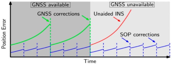
We analyze the increment of the INS-positioning error within 1 s; assuming that the carrier moving speed v = 1000 m/s and the velocity direction error increment Δθ = 1 ’, then the position error increment [10] in the condition of Δt = 1 s is as follows:

Δp = v × Δθ × Δt = 1000 × 1 × 1/60/180 × π = 0.29074 m

(12)

It can be seen that the position error increment of the INS within 1 s is only 0.3 m, even under the assumption of 2.9 times the speed of sound and a large error angle increment. Reference [32] indicates that the LTE-positioning error is generally in the order of 10 m, and the variance value of the error is much larger than the square value of the inertial navigation error increment, satisfying the conditions of Equation (10).

(a): Sliding-window design

In practical applications, considering the stationarity of noise characteristics, the intermediate quantities $Var (Δ Z_{k}^{1})$ , $Var (Δ Z_{k}^{2})$ , and $Var [Δ (Δ Z_{k}^{12})]$ are calculated via statistical sampling, and then the noise variance of the measurement system is estimated using Equation (11).

If all the sampling points are considered, the amount of calculation increases with the increase in the observed amount. When the noise characteristics change, the dynamic information will be submerged in a large number of historical data, and it is not possible to track effectively. Therefore, the sliding-window method is introduced in Figure 8, which can be used to estimate the variance of the first-order difference sequence and the SOMD sequence, considering only the sampling points in the latest time period.

Assuming that the length of the sliding window is

w_{R}

, the variance of the involved random sequence is calculated as follows:

$\{\begin{cases} Var (Δ Z_{k}^{i}) = \frac{1}{k} \sum_{j = 0}^{w_{R} - 1} {[Δ Z_{k - j}^{i} - E (Δ Z_{k}^{i})]}^{2}, i = 1, 2 \\ Var [Δ (Δ Z_{k}^{12})] = \frac{1}{k} \sum_{j = 0}^{w_{R} - 1} {\{Δ (Δ Z_{k - j}^{12}) - E [Δ (Δ Z_{k}^{12})]\}}^{2} \end{cases}$

(13)

where

$\{\begin{cases} E (Δ Z_{k}^{i}) = \frac{1}{k} \sum_{j = 0}^{w_{R} - 1} Δ Z_{k - j}^{i}, i = 1, 2 \\ E [Δ (Δ Z_{k}^{12})] = \frac{1}{k} \sum_{j = 0}^{w_{R} - 1} Δ (Δ Z_{k - j}^{12}) \end{cases}$

(14)

(b): Forgetting-factor design

In order to ensure the real-time noise tracking, the length of the window should not be too long, but it is easy to cause inaccurate estimation results. In order to solve this contradiction, the method of attenuating memory is adopted, and a forgetting factor is introduced to weigh the historical information. The specific steps are as follows:

${\hat{R}}_{k} = (1 - d_{k}) {\hat{R}}_{k - 1} + d_{k} {\hat{R}}_{k}^{-}$

(15)

where

$\{\begin{cases} d_{k} = (1 - b_{k}) / (1 - b_{k}^{k + 1}) \\ {\hat{R}}_{k}^{-} = \frac{1}{2 w_{R}} \sum_{j = 0}^{w_{R} - 1} f (Δ Z_{k - j}^{1}, Δ Z_{k - j}^{2}, Δ (Δ Z_{k - j}^{12})) \end{cases}$

(16)

$b_{k}$ is the forgetting factor, which is used to adjust the use weight of the observation noise variance matrix at the current time, generally 0.95~0.995, ${\hat{R}}_{k}^{-}$ is the direct output of the observed noise variance matrix obtained by SOMD sequence at the current moment, and ${\hat{R}}_{k - 1}$ and ${\hat{R}}_{k}$ are the final estimation results of the noise variance matrix at moment $k - 1$ and moment $k$ , respectively. The function $f (\cdot)$ represents the estimation equation of each algorithm.

(c): Mutation Fault Detection

Considering the real-time nature of the estimation, a finite-length window is used for statistical estimation, so the pollution of the data in the window by the anomalous observations cannot be ignored. In order to suppress the influence of outliers on the estimation of observation noise and improve the accuracy of error estimation, a

k σ

criterion for anomaly data mining [33] is introduced to detect random errors based on SOMD sequence.

In the case of redundant observation

Z_{k}^{1}

and

Z_{k}^{2}

, if there are outliers in any of the observation,

$\{\begin{cases} Δ (Δ Z_{k}^{12}) = (V_{k}^{1} - V_{k - 1}^{1}) - (V_{k}^{2} - V_{k - 1}^{2}) + E r r_{k} \\ ‖Δ (Δ Z_{k}^{12})‖ > \sqrt{Var [Δ (Δ Z_{k}^{12})]} \end{cases}$

(17)

The detection condition of the anomaly can be designed as

$‖Δ (Δ Z_{k}^{12})‖ > κ \sqrt{2 R_{k - 1}^{1} + 2 R_{k - 1}^{2}}$

(18)

where $‖Δ (Δ Z_{k}^{12})‖$ is the modulus of SOMD vector, and $κ$ is the standard deviation coefficient used to judge outliers, called confidence level. The smaller the confidence, the stricter the definition of the outlier, which is usually taken as $κ = 3$ . Due to the stationarity of the statistical properties of noise, the sum of the noise covariance $R_{k - 1}^{1}$ , $R_{k - 1}^{2}$ of the previous moment is substituted for $R_{k}^{1}$ and $R_{k}^{2}$ at the current moment.

As mentioned above, the variance

R_{k}^{2}

of the error in the INS increment is much smaller than the variance value

R_{k}^{1}

of the error in LTE; Equation (18) is simplified to the following:

$‖Δ (Δ Z_{k}^{12})‖ > 3 \sqrt{2 R_{k - 1}^{1}}$

(19)

Equation (19) is the confidence interval of SOP/INS observations. This decision condition can be directly implemented in the SOMD noise estimation process in Section 3.4 without introducing additional data and calculation. According to the correlation between track vector and filter track, the singularities in the SOP pseudo-measurement track can be further filtered out, and accurate system positioning results can be obtained.

3.4.2. RMNCE Validation

An analysis of the effect of the noise covariance with the types and influence factors of the measurement noise is shown in Table 3, generally divided into two cases: case 1 is Gaussian hypothesis distribution; case 2 is time-varying noise distribution, where

V_{k} \sim (0, R_{k})

R_{k}

is the measurement error.

Case 1 is the ideal state,

R_{k}

is the constant, and case 2 is the distribution of measured noise pollution. The variance of the measured noise measured by each observation of the first set of experiments is a fixed value. The variance of the measured noise varies the observed amount over the selected time interval of the second set of experiments. The simulation results of the time-varying noise covariance and observation measurements in the two cases are shown in Figure 9.

The observation data of 600 samples were used to estimate the noise covariance of four redundant measurements under different types, with a sampling interval of 0.01 s. The above two types of noise can be well realized in a real-time tracking estimation of noise covariance when the noise characteristics of the measurement system were unknown or there is no prior knowledge. In case 1, the measurement converges around 20 s, and the SOMD estimation results converge around the true value quickly; in case 2, the measurement noise variance had been changed between 100 and 450 s, and SOMD can effectively sense the change and realize the estimation of noise covariance. At the same time, case 2 illustrated that the estimations of the noise variance of each dimension of the measurement system by the SOMD algorithm were independent of each other and were not affected by the measurement noise of the other dimensions. The positioning error can be estimated by inputting the above adaptive measurement noise covariance into the navigation model.

Meanwhile, the observation data of 600 samples were used to estimate the noise covariance under different forgetting factors. The measurement 2 parameters in Table 3 were selected to estimate the measurement noise, and the forgetting factors were 0.95, 0.97, and 0.99, respectively. Figure 10 shows the variance of noise covariance. As can be seen from the figure, the larger the noise, the closer was to the real noise, and the estimation effect of noise covariance was better when the factor was 0.99.

3.4.3. EKF Framework

For the navigation system, it can be regarded as consisting of two parts, one of which is correctly predicted by the known motion equation, and the other as a random component with zero mean. Considering the difference in INS/SOP integration architecture, the EKF, the unscented Kalman filter (UKF), and the particle filter (PF) are usually used and other nonlinear filters to deal with the nonlinearities of the integrated system. Although the UKF algorithm appears to have considerable advantages over the EKF method, the unknown statistical properties of noise are still a stumbling block to its optimal estimation [34]. Different from the UKF method, which is based on deterministic sampling, the PF method applies a large number of random particles to approximate the posterior density distribution of the state [35] and even requires a heavy computational burden and faces particle degradation and sample poverty in practical applications usually [36]. Since the observed vectors are usually uncorrelated in each dimension, the SOMD algorithm can be used separately in each dimension.

The simulation scene was set where the X–Y axis target moves along a straight line at a constant speed, and the positioning performances using EKF and PF algorithm before and after proposed RMNCE are analyzed. The simulation parameters are seen in Table 4.

Figure 11 shows the simulation results of filtering track and error based on EKF and PF algorithm. From the analysis of positioning accuracy, it can be shown in Figure 11a, the PF track was closer to the real track, which had obvious advantages, and the positioning RMSE can reach 0.42 m, due to the particles of the PF can be reset after each measurement updating. Considering RMNCE, the positioning accuracy of the two filters had been partially improved, among which the positioning effect of RMNCE PF was better than that of RMNCE EKF; however, the accuracy was higher in several areas, such as Y-axis RMSE, due to the weighting factor of PF being related to the measurement noise and the measurement noise changing constantly. It can be difficult to sample the real distribution, and it occasionally diverged or even failed. From the calculation time, the number of particles used by PF occupies a certain scale; it takes about 30 s for PF and RMNCE PF to process a 500 m measurement track. However, EKF and RMNCE are much faster than 0.01 s, which is obviously advantageous for the real-time navigation. Table 5 was an overview of the simulation time and positioning error of the filters. The above simulation results are ideal, which shows that RMNCE has certain advantages. However, the applicability of this algorithm to most real-world systems is limited because it relies on redundant measurements.

The research in reference [37] shows that deep learning and other methods can be used to predict the motion state of the carrier more accurately, but considering the computing power and complexity constraints of the platform, EKF is commonly used to estimate and filter. In this paper, the EKF framework based on RMNCE is used to deal with the measurement track.

Source link

Li Zha www.mdpi.com

Greenberg News

Robust Regression and Redundant Measurement Noise Estimation Adaptive Filtering for Localization in Urban Environments

3.4.1. SOMD Noise Estimation

3.4.2. RMNCE Validation

3.4.3. EKF Framework

Greenberg

3.4.1. SOMD Noise Estimation

3.4.2. RMNCE Validation

3.4.3. EKF Framework

Related Posts

Environmental Factor – August 2020: National Academies forum links chemicals to brain disorders

Improving Physically Unclonable Functions’ Performance Using Second-Order Compensated Measurement

Environmental Factor – August 2020: Distinguished Lecture explores social-genetic effects in fish

Greenberg