
1. Introduction
A common feature of most of the previous research in this area is its abstractness and difficulty for practical implementation. The purpose of the present study is to develop and deploy a calculation framework for the economic costs and environmental burdens for domestic waste collection, also considering relevant social factors. The framework allows many different scenarios covering multiple issues to be considered in conjunction with trade-offs and sensitivities of most interest. In turn, this informs decision-making, mostly at the operational level but occasionally with more strategic elements. The result is a framework more widely applicable and flexible than normally appears to be the case. One key consideration in model development and implementation is the trade-off between flexibility and general applicability of the model, and the extent and resolution of data required for the model. Most studies reported in the literature appear relatively specific and limited in scope.
2. The Calculation Model
The model evaluates economic costs, environmental impacts, and social factors for domestic waste collection operations. The model simply analyses costs and does not consider how these are met in practice. For example, the levels of municipal taxes levied on residents are not considered. In the interests of flexibility and generality mentioned above, many of the parameters listed below are used on a relatively averaged and/or general basis.
2.1. Model Inputs and Outputs
The model calculates the following principal outputs for a given collection duty:
The total economic cost (per tonne) broken down into fixed, variable, and staff costs.
The total environmental impact and the impact per tonne.
The operational efficiency in terms of the average degree of filling of collection vehicles and of customer kerbside solutions such as bins. These operational efficiencies present constraints in the calculations—neither bins nor vehicles are allowed to become over-filled.
The breakdown of operational time into driving, the emptying of bins and the emptying of vehicles. This allows the effects of potential changes to the operation to be assessed to see if the emptying of bins could be made quicker on average by deploying more staff, for instance.
The principal inputs to the model are as follows:
- Waste generated/collected: it is recognised that most data for waste collection are presented in mass terms—see [29], for example. However, the practical reality is that vehicle loading and operation is limited by volume rather than mass. Hence, although the model uses mass terms for the original waste generation, this is converted to volume using values for typical (kerbside) bulk density.
The collection vehicle design: as mentioned above, the collection duty is assumed to be fulfilled by a fleet of identical vehicles. The vehicles are permitted to have one or two chambers, each with specified volume and each allowed to compress waste by a specified factor. Vehicles can be driven by diesel, biogas, or electricity. The working lifetime of vehicles drives economic and environmental costs.
The number of collections per annum: by default, the model considers calculations on an annual basis, but the model would work equally well for single collections or shorter periods by scaling the waste collected and number of collection values appropriately.
- The total annual driven distance: this was considered at length in the development of the model. It can, in principle, be calculated via detailed network mapping and vehicle routeing calculations—an illustrative example for a model similar to the present study is provided by [30]. However, it was decided to simply consider the total driven distance as known within the model. The distance required is the distance for one complete collection round—visiting every household in the region once. Our experience with working with municipality data was that terminology is often unclear; words such as “trip” were used ambiguously.
The average driving speed: as the model is constituted, the parameter represents the average speed for all the time the vehicle is moving, both when going to and from the collection area, where it is relatively high, and when moving from household to household within the collection area, where it is obviously low.
The time per bin emptied: this is once again entered in the model as an overall average, although in practice the emptying time will vary with the type and size of bin, the type of loading (for example back-loading or side-loading, with a crane or otherwise), the aptitude of the personnel on the vehicle, the physical location of bins relative to roadside, and so on.
The time for return and emptying of full vehicles: our investigations showed that operational patterns for collection vehicles varied greatly, depending, for instance, on geographical or demographic patterns. In some cases, vehicles could require emptying several times per day, whereas in sparsely populated remote regions, vehicles could operate for several days before requiring emptying.
The number and size of bins: these data are used directly in the calculation of costs relating to infrastructure. The number and size of available bins establishes a total kerbside available volume, which in turn is used in conjunction with the average volume of waste per emptying to give the average degree of filling of bins.
- Cost factors: these are the capital investment in the vehicles, and annual fixed costs for administration, ferries and tolls, and taxes and fees. Variable cost factors include the cost of fuel, fuel efficiency, and cost estimates for vehicular repairs, maintenance, and tyre replenishment. All these factors are presented very similarly to previous work [13].
Staffing: the model allows for staff to be deployed on an annual retained employee basis, as typical for in-house operations, or on an hourly paid basis as typical for contracted-out work. An average staff cost (per annum or per hour) is required, along with an average number of staff per collection vehicle.
2.2. Calculations: Logistical Factors
The central driver for economic costs is the operational time required to undertake the major parts of the operation (driving, emptying bins at kerbside, and emptying vehicles when full). The calculations begin with the time required to empty bins.
where M is in tonnes, V is in m3, and ρ is in kg/m3. The total number of times the vehicle must be emptied, E, in collecting this volume of waste depends on the volume of the chamber, C, the compression factor R and the average degree of filling, f:
where Ei is the number of emptyings that would be required based on chamber i. The denominator of (2) gives the effective volume available for collection in the chamber. For example, a 15 m3 chamber compressing its intake threefold but only being filled 80% full on average has an available volume of 15 × 3 × 0.8 = 36 m3. In practice, the vehicle is assumed to be emptied whenever any chamber reaches this limit, so E for the vehicle is the maximum value of Ei across both chambers. This in turn allows for the total operational time for emptying of the vehicles to be calculated. This incorporates return of the vehicle to the depot and the emptying process:
where Tvehicle is the total time for all emptyings and t the average time of each emptying (known). Next, the model calculates the time for driving. This is a simple function of the overall distance driven and average speed (S, in km/h), the distance driven depends on the number of collections per annum (A) and the distance in km required for each collection (D):
where tbin is the average time for emptying a single bin. The number and volume of bins establishes a maximum available bin volume for each collection round. The average degree of filling, an important service parameter, can thereby be calculated:
where (V/A) is the actual volume of waste collected per collection, and (B. VB) is the total available volume in all bins. The total operational time for an annual period is the sum of the three parts in Equations (3)–(5). This in turn is used to determine the number of vehicles necessary to fulfil the collection duty, as described above. If Tmax is the maximum allowable annual operational time and is shared equally between N vehicles:
where the second term is the integer number of vehicles required, rounded down. The vehicle and staff utilisation factor U, giving the fraction of a full annual operational schedule used by each vehicle and its crew, is given by
where (Tvehicle + Tdriving + Tbin)/N is the total operational time for each vehicle in the fleet.
2.3. Calculations: Cost Factors
where (A.D) is the annual driven distance in km, efuel the fuel use per km and Pfuel the unit cost of fuel. The fuel can be diesel, electricity or biogas so long as the relevant unit cost and average fuel efficiency are known. Finally, the staff cost is calculated as
where N is the number of vehicles, Sveh the average number of staff per vehicle (which can be non-integer if the vehicle duty combines parts with different numbers of staff as sometimes occurs), and PUstaff is the unit staff cost. If staff are deployed on an annual deployed basis, PUstaff is simply a known parameter capturing the average cost of staff (including salary and any indirect costs), whereas for hourly based staff the unit value is multiplied by the annual number of hours worked, which is 1875 by default.
2.4. Calculations: Environmental Factors
where Xvehicle is the impact of producing one vehicle, Xfuel is the impact of producing and consuming one unit of fuel (litre of diesel or kWh of electricity), and Xbins is impact of producing bin of unit size (one litre). The latter is averaged over bins of different sizes; calculations show the raw material per litre of provided volume is almost constant. Hence, the third term of Equation (13) captures the production of all the bins for the required collection.
3. Case Study Description
The case study presented concerns the co-collection of residual waste and biowaste in a mixed urban–rural community of around 120,000 inhabitants. The collection duty is fulfilled by a fleet of identical two-chamber vehicles. Collection is limited by the operational time needed for its completion, which is calculated and expressed in vehicle-hours. Calculations are first performed on a total annual basis. However, collection duties in practice vary on a shorter-term (daily or weekly) timescale, depending on factors including road conditions and waste generation which vary seasonally and naturally fluctuate. An important part of the analysis concerns examining these fluctuations and operational sensitivities.
Many of the annual average data have been measured directly. Collection is found to require around 220,000 km of driving or 4231 km per collection for 52 collections per annum. Specifically, this distance is that required to visit each and every household in the area, along with the requisite transport to and from the depot. The transport is completed at an annual distance-averaged speed of 18.6 km/h, based on the proportions of the total distance to, from, and within collection areas, and the average vehicle speeds. Across the two waste fractions, around 20,000 tonnes of waste per annum is generated (13,163 tonnes of residual waste and 7200 tonnes of biowaste). The two fractions combined are collected via an array of 63,950 waste bins, varying in size from bins typically suitable for a single household of 120–140 L, to communal bins for multiple households of up to 1000 L.
Each household in the community is visited weekly; however, collection is expected to be somewhat flexible and on-demand and only half of all bins are emptied in any given week on average. The municipal levies for collection reflect this (individual consumers can choose different arrangements and pay accordingly), although the funding of the operation is not considered directly in the case study and such operational differences are averaged out. The emptying of each bin takes 19 s on average. Emptying the collection vehicle at the depot takes an average of 15 min, according to the supplied data, and this occurs roughly once daily. The vehicle is sent for emptying whenever either chamber is full and depends on the relative size of the chambers, the bulk density of the waste, and the compression of the waste in-vehicle. In practice, the emptying of the vehicle is limited by collection of biowaste rather than of residual waste.
The annual operational time breakdown is as follows. Around 55% of the total time is for driving, 41% for bin emptying, and 4% for vehicle emptying.
Each collection vehicle is assumed to support one working shift (37.5 operational hours for 50 weeks per year, hence 1875 total operational hours). Therefore, the total fleet size is 21,401/1875 = 12 vehicles (naturally, the fleet size is rounded-up to the higher integer). As will be shown, the fleet size is a key driver for both the environmental and economic costs of collection.
4. Results: Sensitivity to Conditions and Operational Parameters
The calculation model allows for the following parameters to be varied: the design of the collection vehicles (number and size of chambers, compression ratio in-vehicle, and criteria for emptying), the mass of wastes generated per annum, the frequency of collection, the driving distance per collection, the average speed, the number of bins of different sizes and the fraction emptied each time, the time per bin emptying and vehicle emptying, and the crewing of vehicles. Financial and environmental parameters such as the important cost drivers and fuel economy will be considered separately below.
Some parameters are held constant across most or all analyses. These are generally factors that might be considered strategic rather than tactical or operational—the present study is focused on the latter. Strategic parameters include the dimensions of collection vehicles and the driving distance per collection. Neither of these are expected to change often, if at all. The former would require significant capital investment and the latter is taken to have reached a practical optimum, constrained by the local geography, and assumed immutable factors such as depot locations. Whilst factors such as optimal vehicle routeing remain a widespread area of research, they are not considered here.
4.1. Sensitivity to Variation in Waste Generation
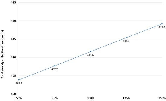
Waste generation naturally varies between households and also seasonally. As noted above, it is perhaps more appropriate to conceive fluctuations on a daily or weekly basis. Since most collection in practice is on a weekly or multiple-weekly schedule, the calculation model is readily scalable from an annual to a weekly basis, and the latter is considered in the following calculations.
As outlined above, the modelling of domestic solid waste generation is a large research field. However, most studies are highly location-specific and general information on seasonal fluctuation in waste generation could not be identified. Nor were specific data available here. Hence, a conservative range of generation rates, attempting to capture all realistic possibilities was considered; the weekly rate was allowed to vary between 50% and 150% of the annual weekly average.
However, the analysis ignores one key factor, this being the (average) fullness of bins when they are emptied. This factor brings into focus the major trade-offs to be considered in this scenario. The calculations shown assume that 50% of all bins in the area are emptied per visit, irrespective of the waste generation level. This factor has implications for the service level provided to consumers and for the efficiency of collection. Bins should be emptied sufficiently often that the risk of overfull bins is rather low, but near-empty bins on collection signifies that collection may be too frequent and hence inefficient, especially economically. Variations in waste generation from household to household probably mean that the possibility of overfull bins on collection can never be completely eliminated, but this should clearly be reduced to a low level. The base case where the waste generation level is 100% of the average gives rise to an average bin fill at collection of 51.3%, calculated from the volume of waste generated divided by the available volumetric bin capacity. This seems reasonable for allowing considerable variability in fill from bin to bin whilst still making overfull bins quite unlikely.
The average bin fill scales with the waste generation level. So, for example, if it were doubled from the base case then most bins would be overfull (the average bin having a fill of 102%); this would clearly be an unacceptable service level for consumers. In the example presented here, the maximum 150% waste generation level gives an average bin fill of 77% which would suggest a significant number of overfull bins. At the 50% waste generation level, the average bin is only 25% full on emptying, and this is likely to drive up costs of collection (considered further below).
4.2. Sensitivity to Driving-Related Parameters
The two main driving-related parameters are the distance and the average speed. Base case numbers are gathered directly from the waste collection operator. The distance per collection round of 4231 km is measured directly from vehicular data. The distance-averaged speed of 18.6 km/h arises from the observation that 45% of all vehicle-kilometres are inside the collection area and 55% outside, with average speeds of 10 km/h and 60 km/h, respectively. These are annual-averaged figures with an obvious short-term sensitivity to factors such as road conditions and weather. Only annualised data were available; hence, estimates for shorter-term fluctuations in these parameters are necessary. It is assumed that the driving distance is an unchanging feature of the local geography. The average speeds could certainly vary with factors including weather and traffic congestion. It perhaps seems reasonable that the low average speed within the collection area is relatively stable in different conditions, but that the higher speeds to and from the area could vary. This means that the overall averaged speed is relatively insensitive to change. If the higher speed is allowed to fall from 60 km/h to 40 km/h, the overall distance-averaged speed falls relatively little, from 18.6 km/h to 17.1 km/h. This would add about 20 h (5%) to the weekly collection time and hence necessitate the addition of a twelfth vehicle to the fleet.
4.3. Sensitivity to Emptying Times
In the base-case scenario, there are around 60 vehicle emptying events and around 30,000 bin emptying events each week; hence, the total operational time would be expected to be somewhat sensitive to the emptying times. It seems unlikely that vehicle emptying times could vary much from existing values. The relevant processes, such as arriving at the depot, finding a suitable location, emptying the vehicle, and departing, are probably relatively streamlined and largely invariable. In contrast, the bin emptying time could be sensitive to a range of factors, such as the size and type of bins, the type of loading (back-loading or side-loading, with a crane or otherwise), the physical positioning of bins relative to roadside (in turn depending on factors such as the housing stock and the behaviour of consumers in terms of placing their bins), the crewing of collection vehicles and the aptitude of staff, and so on.
Because of the large number of events (30,000 per week or nearly 1.7 million per year), a small difference in average bin emptying time can have a noticeable effect. From the base-case value of 19 s, each second difference in average bin emptying time varies the weekly total collection time by about 8 h. To relate this to the variables considered previously, an 8 h difference in weekly collection time arises from a change in waste generation of about 5% or a variation in the higher driving speed of around 10 km/h. It is literally the case that “every second counts” with respect to bin emptying. It is possible to imagine that the bin emptying time could be influenced by elements including staff training and/or performance-related objectives, and also communication with customers to encourage the proper placement of bins kerbside. The efficacy of any such measures will also depend on the financial elements (see below).
4.4. Sensitivity to Infrastructural Elements (Economies of Scale in Bin Provision)
All of the calculations so far are based on a particular infrastructure, in terms of a total number of bins of particular volumes that serve the households within the community. The efficiency of collection could in principle be influenced by a greater use of communal bins across more households, thus reducing the total number of bins to be emptied at any given time. It is assumed that this is only feasible for residual waste; the number and size of bins for biowaste collection are left unaltered. Any consolidation of bins resulting in householders no longer having their own effectively represents a drop in service level, but if bins do not become overfull then the effect might not be too great.
In the scenario as configured, there are around 34,000 bins of various sizes for residual waste, which provide a total volume of 6.126 million litres. Leaving aside issues of practicality, this could in principle be consolidated into an array of 6126 bins of 1000 litre capacity (the largest in the existing system) to provide the same total available volume. Were this possible to implement, the economies of scale for the bin emptying time in particular would be considerable. The total weekly collection time across both waste fractions would fall from 411.6 h in the base case scenario to 337.6 h, or by around 18%. This is a considerable reduction, which would correspond to the effect of waste generation falling by nearly 40%. The change arises purely from bin collection time differences. In principle, the driving distance or time might also fall somewhat, but this is not considered here. The total consolidation of bin provision described is clearly unrealistic, but the calculation indicates that any economy of scale of this sort is potentially valuable.
4.5. Sensitivity to Vehicle Operations and Crewing
A second possible operational change is to vary the crewing of individual vehicles. In the present base-case scenario, there are two crew per vehicle. It is possible to conceive driver-only operation. In this case, the driver must leave and re-enter the cab at each stopping point, also retrieve and return the bins individually, whereas in a double-crewed operation, the driver may or may not retrieve at any given stopping point. The time per bin emptied will clearly increase for driver-only operation, and this increased time burden may ultimately necessitate an increased number of vehicles. This would be traded-off against the reduction in staff costs per vehicle.
Limited trial evidence suggests that the bin emptying time increases from 19 s to around 30 s per bin in single-driver operation. As the above calculations suggest, this would give rise to a substantial increase in bin emptying and hence overall collection time from 411.6 h to 509.3 h per week, an increase of nearly 24%, which equates to the effect of increasing waste generation by over 50% from the base case. The total fleet size requirement would rise from 11 to 14 vehicles, although each would be single-crewed.
4.6. Economic Effects
4.7. Climate Change Effects
4.8. Summary Calculations for Rural Collection
The calculations shown are for a semi-urban area of around 120,000 inhabitants. For broad comparison, summary results are shown for a more remote location, where the majority of the 15,000 residents are located in the most important small town, but the remainder are highly dispersed over a wide area where the opposite ends are separated by more than 60 km. Some additional operational differences are in evidence (the size and distribution of bins is quite different) but the local geography is the defining difference between the two scenarios. The collection of 2500 tonnes of waste requires around 3000 h of operational time hence around 60 h per week, and a fleet of two vehicles is required. Each bin is emptied every two weeks, with an average fill at emptying of around 67%; hence, there is a significantly higher risk of overfull bins than for the previous scenario.
For climate impacts, the picture is broadly as might be expected. Climate impacts are higher for the rural collection, but not hugely so since the driving distances per tonne of waste collected are not massively higher. The base case gives an impact of around 27 kg CO2 equivalent per tonne collected. Once again, this is only significantly influenced by a change to electric vehicles.
5. Discussion
The development of the model has highlighted key issues relating to the flexibility and generality of modelling approaches to cost/environmental analysis of domestic waste collection. Models in the literature, and those presented by interested parties in the research project in which this study was housed, are typically very specific and inflexible. Large numbers of adjustable parameters, presenting severe problems in terms of data-gathering (and some risks regarding credibility), are a common feature. This work has attempted to address some of these issues by formulating a model with relatively few adjustable parameters. It remains quite heavily dependent on specific data and assumptions-reconciliation with such data that is typically available to potential users of such models remains important. Nonetheless, it is possible to explore some general sensitivities and parametric relationships in ways that is not always possible or easy with models of this sort.
The results suggest that staffing accounts for most of the costs (70–90%) in both urban and rural environments. Downward cost pressures are best directed at reducing operational time. Each tonne of waste collected implies driving long distances, often at low average speeds where vehicles are starting and stopping at very short intervals. Observing waste collection operations suggests there is probably little potential for improvement in this respect and operatives normally appear highly experienced and efficient in navigating the appropriate routes. There may be some scope at the more strategic level through the reorganisation or reconfiguration of vehicle routes; this is obviously an important area of research in its own right. These could serve to reduce the necessary driven distance per tonne of waste. The collection and emptying of bins may account for 30% or more of the total operational time. As discussed above, to some degree this will depend on the aptitude of crews, and recruitment/training may have a part to play. Encouraging positive consumer behaviour, for instance the placing of bins appropriately at kerbside to facilitate rapid emptying, could be a relatively low-cost possibility for achieving some improvements. The routeing and scheduling of vehicles may also facilitate reductions in time for vehicle return to depot and emptying. The model highlights tipping points at which cost levels can undergo stepwise changes, particularly where changes in operations lead to changes in the numbers of staff or vehicles. Such points are probably less sharp in practice than the model suggests but should still be borne in mind. More generally, the need to use both vehicles and staff efficiently is very clear in the model.
Most operations are still performed by diesel-fuelled vehicles and in this case, fuel is almost always the most significant driver of environmental burdens associated with domestic waste collection, accounting for perhaps 70% of all climate change burdens. The manufacture of bins is a stronger contributor to total burdens than one would perhaps intuitively expect. In the scenarios presented in the paper, it can account for a third of climate change potential. It appears that climate change potential is relatively insensitive to many operational changes. Improving fuel economy is an obvious possibility but otherwise, a radical reorganisation of operations to reduce driving distances may be required. Switching to electric vehicles where possible has an obvious potential for reduced emissions; the small environmental burdens because of the increased complexity of the vehicles are easily outweighed by the emissions savings from electric power. The burdens associated with waste bins can be substantially reduced by the use of recycled plastic.
6. Conclusions
This paper has described a model for economic and environmental burdens of waste collection that is highly flexible and is beginning to be used by interested parties. It offers research insights into the sensitivities and dependencies of cost and environmental factors to operational parameters. It has been used both to highlight parameter sensitivities, in general, and to answer specific questions of interest. Ongoing work includes the gathering of further data for more refined parameterisation of the model. The intention is not to “correct” the shortcomings of the modelling approach in terms of its generality, but to gather better estimates of the (often approximate) parameters in the model as it stands.
Source link
Eirill Bø www.mdpi.com