2.1. Desalination Plant
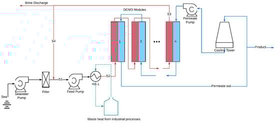
Figure 1 illustrates a schematic diagram of the hypothetical seawater desalination plant. The proposed plant operates in a constant recovery mode, where a portion of the concentrated brine (stream S3) is discharged from the system, while the remaining portion (stream S4) is recycled back into the process. This recycling process enhances thermal efficiency and increases water recovery [
18].
The process begins with seawater, containing a salt concentration of 3.5 wt.% and an ambient temperature of 20 °C, passing through a filtration system to remove suspended solids. The filtered seawater is then mixed with the recycled brine stream (S4), resulting in an increase in both the temperature and salt concentration of the feed water.
The outlet feed stream from the MD modules is set to reach a salt concentration of 25% (
w/
v), which is maintained below the salt saturation limit of 35% at 20 °C to prevent salt crystallization within the system. This feed outlet concentration supports a water recovery ratio of 83%, calculated as the volumetric flow rate of the product water divided by the volumetric flow rate of the seawater entering the plant [
19].
Stream S1 is directed into the HX-1 heat exchanger, where it is heated using available waste heat until reaching the desired feed inlet temperature (
Tf,in). Potential sources of waste heat include return cooling water from petrochemical industries, flue gases, or steam. However, specific details about the waste heat source are excluded to allow for a more generalized cost analysis. While this study assumes waste heat to be freely available, we acknowledge that heat sources above 80 °C may not always be accessible at no cost. However, as demonstrated by Jantaporn et al. [
20], the specific energy requirement for DCMD is primarily dependent on the recovery factor, not membrane properties, so thermal energy consumption is excluded from the cost analysis, focusing instead on other cost-contributing factors.
Once heated, the feed enters the membrane distillation (MD) modules as stream S2 to achieve the target concentration. The cold stream is introduced into the MD modules in a counter-current flow configuration to maximize the temperature gradient, exiting at the opposite end. Afterwards, the cold flow undergoes further cooling via a cooling tower or pond.
Table 1 summarizes the membrane and module specifications used in this study. A plate-and-frame MD configuration was selected, as it enables higher flow rates, thereby enhancing water flux [
21]. Each module is equipped with a suitable mesh spacer to promote fluid mixing and includes a total membrane area of 1.25 m
2.
To improve channel length, membrane area, and hot stream residence time, the membrane modules are arranged in a combination of series and parallel configurations. However, increasing the channel length can reduce mass flux across the module due to a decreased driving force. Therefore, it is necessary to optimize the membrane length to achieve the best performance. In this study, the optimal configuration includes five membrane modules connected in series, resulting in a total membrane area of 6.25 m2 for each cascade with a counter-current flow.
2.2. Mathematical Modeling of DCMD
To evaluate the effects of membrane surface hydrophobicity and pore size on the performance of DCMD, a comprehensive model was developed to simulate the coupled heat and mass transfer processes.
Figure 2 provides a schematic representation of the DCMD process operating in a counter-current configuration [
22].
The transmembrane mass flux
J (kg·m
−2·s
−1) is described by the equation below:
The MD coefficient
C (kg·m
−2·s
−1·Pa
−1) depends on various factors, such as membrane characteristics, vapor properties, and membrane surface temperatures [
23]. The water vapor pressures at the membrane surfaces on the feed and permeate sides, denoted as
pf,m (Pa) and
pp,m, respectively, are calculated using the Antoine equation based on their corresponding surface temperatures [
22]:
where T (°K) and p (Pa) are the membrane surface temperature and water vapor pressure, respectively. The water vapor pressure at the feed side, pf,m, is lowered due to the presence of dissolved salt, with the mole fraction of xs,f, as described by Raoult’s law, which is expressed by the following Equation (3) [24]:
where (Pa) is the vapor pressure for pure water with no dissolved species.
The mean pore size of the membrane plays a significant role in determining the mass transfer mechanisms through the porous membrane [
25]. The Knudsen number (
Kn), as given by Equation (4), is a crucial parameter that determines the dominant mass transfer mechanism through the pores [
23]:
where
dp (m) is the membrane pore diameter, and λ (m) is the mean free path of gas molecules across the pores. Depending on the value of
Kn, the mass transfer through the pores can be dominated by transition, Knudsen diffusion, or molecular diffusion mechanisms. Specifically, for
Kn values less than 0.1, the mass transfer is dominated by convective flow and molecular diffusion in the transition regime. For
Kn values between 0.1 and 10, Knudsen diffusion, characterized by gas molecules bouncing between pore walls, becomes the dominant mass transfer mechanism. For
Kn values of greater than ten, molecular diffusion, with gas molecules diffusing through the pores without any collisions, dominates the mass transfer process [
26]. For membranes featuring pore sizes smaller than 0.5 μm, a typical pore diameter for membranes in MD systems, the combined Knudsen/molecular diffusion model is typically applied, and Equation (5) is used to determine the MD coefficient [
26,
27]:
Wherein, the parameters
r (m),
δ (m),
τ, and
ε represent the average pore radius, thickness, tortuosity, and porosity of the membrane, respectively.
Mw (kg·kmol
−1) denotes the molecular weight of water,
Dw-a (m
2·s
−1) signifies the water vapor diffusivity in air, and
R (J·kmol
−1·K
−1) represents the gas constant.
Pa (Pa) and
P (Pa) are the air pressure and total pressure in the membrane pore, respectively. Meanwhile,
(°K) represents the membrane mean temperature, which can be obtained from Equation (6) [
26]:
where Tp,m and Tf,m (°K) are the surface temperatures of the membrane at the permeate flow and feed sides, respectively. Dw-a is determined by Equation (7) [23]:
The membrane distillation coefficient, as described by Equation (5), is significantly influenced by the properties of the membrane, including pore size, porosity, thickness, and tortuosity. Among these properties, thickness and pore size are likely to have a more dominant effect on permeation, as porosity and tortuosity tend to fall within a narrow range [
14].
In a steady state, heat transfer in DCMD involves three main components: convective heat flux through the feed boundary layer (
Qf), the combined conductive heat flux and latent heat associated with mass flux through the membrane (
Qm), and convective heat flux through the permeate flow boundary layer (
Qp). The mathematical expressions for these heat transfers are presented in Equations (8)–(10) [
28]:
The heat transfer coefficients on the permeate flow and feed sides, denoted as hp and hf (W·m−2·K−1), respectively, are calculated using appropriate empirical correlations. Tp and Tf (°K) represent the average temperatures of the permeate flow and feed bulk, respectively.
The vaporization enthalpy at the membrane mean temperature is denoted as Δ
Hv (J·kg
−1) and can be obtained from [
29].
The membrane thermal conductivity,
km (W·m
−1·K
−1), is determined using Equation (11), which involves the thermal conductivities of the gas in the pores,
and the membrane polymer,
kp, respectively [
30]:
The conductive heat transfer through the membrane is considered as heat loss. Equation (12) is utilized to determine the thermal efficiency (
η) of the MD process, which represents the fraction of the total heat transferred through the membrane that is associated with the mass flux [
10]:
By considering the overall heat balance in the steady state (
), the surface temperatures of the membrane can be calculated using Equations (13) and (14) [
4]:
The temperature of the membrane surfaces deviates from the bulk temperatures, which is referred to as temperature polarization, and the temperature polarization coefficient (
TPC) can be determined using Equation (15) [
31]:
The heat transfer coefficients
hf and
hp are determined using appropriate empirical correlations based on the flow regime (laminar or turbulent) within the membrane channel, as described in Equations (16)–(18) [
30]:
where Pr, Re, and Nu represent the Prandtl, Reynolds, and Nusselt numbers, respectively, and k (W·m−1·K−1) and Dh (m) denote the liquid thermal conductivity and the hydraulic diameter of the module, respectively.
2.6. Cost Calculation
The water production cost (WPC) of a desalination plant is influenced by various factors, including plant capacity, lifespan, feed water quality, pretreatment requirements, process technology, and energy costs [
33]. In this study, the WPC for the proposed desalination plant was estimated based on the total capital costs (TCCs), which included equipment, instrumentation, and control costs. Additionally, annual operating costs, such as energy consumption and membrane replacement, were considered [
26,
33,
34]. Land costs were excluded from the calculations, as MD systems typically require a small footprint. The data and assumptions used in the WPC calculations are summarized in
Table 2.
The cost of the hydrophobic PVDF membranes used in this study was assumed to be
$60/m
2, which is comparable to the reported cost of PTFE membranes in previous research [
35]. The membrane cost was considered to constitute 33.3% of the total cost of the membrane module, including both the cost of membrane itself and its assembly. Therefore, each MD module, with a membrane area of 1.25 m
2, was estimated to cost
$225, based on the criteria outlined by Banat and Jwaied [
33].
The purchase cost of pumps was determined based on the required shaft power and referring to the cost curve for cast iron centrifugal pumps found in the literature [
36]. Similarly, the purchase cost of the heat exchanger was calculated by considering the required heat transfer area, derived from simulation results, and referring to a specific cost curve tailored for fixed tube sheet heat exchangers with a carbon steel shell and tube design [
36]. To account for inflation, the estimated costs of pumps and the heat exchanger were adjusted to the Chemical Engineering Plant Cost Index (CEPCI) of 1982, then converted to the year 2019 using the most recent CEPCI available at the time of the analysis. The membrane cost was estimated based on the required membrane area, determined from the plant’s production capacity and the DCMD water flux. The annualized capital costs (
$/year) were calculated by multiplying the total capital costs (TCCs) by the amortization factor presented in Equation (20), assuming a 5% interest rate for borrowed funds [
33].
where i (%/year) represents the annual interest rate, and n (years) represents the expected plant lifetime.
The yearly operating cost in this study is calculated based on the annual energy consumption, with an assumption of 20% membrane replacement per year. In MD plants, the required thermal energy is a major contributor to the WPC, as stated in previous studies [
35]. To meet this thermal energy requirement, it is assumed that any available waste energy is utilized. This is commonly feasible in industrial plants that generate cooling or hot streams as discharge, as suggested in [
26]. Therefore, the energy requirement in this study is primarily limited to the electricity consumption for pumping,
, which can be calculated using Equation (21):
where
qv (m
3/s) and Δ
P (Pa) represent the flow rate and the pressure difference in the pump, respectively. The pump efficiency, denoted by η, is assumed to be 65%. The desalination plant is assumed to operate continuously throughout the year. To calculate the annual electricity cost (
$/yr.), the electricity consumption is multiplied by the specific electricity cost (
$/kWh) and the total number of operating hours per year (24 h/day × 365 days/year × plant availability factor).
The
WPC (
$/m
3product) is then determined by adding the amortized
annual capital cost (
$/yr.) and the
annual operating costs (
$/yr.) and dividing the sum by the
annual production (m
3product/yr.), as expressed in Equation (22):